damp
Natural frequencies and damping factors.
Syntax
[wn,z] = damp(sys)
[wn,z] = damp(P)
[wn,z] = damp(P, dt)
[wn,z] = damp(R)
[wn,z] = damp(R, dt)
Parameters
- sys
A linear dynamical system, in state space, transfer function or zpk representations, in continuous or discrete time.
- P
An array of polynomials.
- R
An array of real or complex floating point numbers.
- dt
A non negative scalar, with default value 0.
- wn
vector of floating point numbers in increasing order: the natural pulsation in rad/s.
- z
vector of floating point numbers: the damping factors.
Description
The denominator second order continuous time transfer function
with complex poles can be written as s^2 + 2*z*wn*s + wn^2 where z
is the damping factor and wn the natural pulsation.
If sys is a continuous time system,
[wn,z] = damp(sys) returns in wn the natural
pulsation ωn (in rad/s) and in z the damping
factors ξ of the poles of the linear dynamical system
sys. The wn and
z arrays are ordered according to the increasing
pulsation order.
If sys is a discrete time system
[wn,z] = damp(sys) returns in
wn the natural pulsation
ωn (in rad/s) and in z the
damping factors ξ of the continuous time
equivalent poles of sys. The
wn and z arrays are
ordered according to the increasing pulsation order.
[wn,z] = damp(P) returns in
wn the natural pulsation
ωn (in rad/s) and in z the
damping factors ξ of the set of roots of the polynomials
stored in the P array. If
dt is given and non 0, the roots are first
converted to their continuous time equivalents.
The wn and z arrays are ordered
according to the increasing pulsation order.
[wn,z] = damp(R) returns in
wn the natural pulsation
ωn (in rad/s) and in z the
damping factors ξ of the set of roots stored in the
R array.
If dt is given and non 0, the roots are first
converted to their continuous time equivalents.
wn(i) and z(i) are the the
natural pulsation and damping factor of R(i).
Examples
s = %s;
num = 22801 + 4406.18*s + 382.37*s^2 + 21.02*s^3 + s^4;
den = 22952.25 + 4117.77*s + 490.63*s^2 + 33.06*s^3 + s^4
h = syslin('c', num/den);
[wn,z] = damp(h)
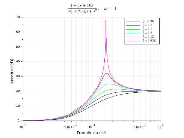
The following example illustrates the effect of the damping factor on the frequency response of a second order system.
s = %s;
wn = 1;
clf();
Z = [0.95 0.7 0.5 0.3 0.13 0.0001];
for k=1:size(Z,'*')
  z = Z(k)
  H = syslin('c', 1 + 5*s + 10*s^2, s^2 + 2*z*wn*s + wn^2);
  gainplot(H, 0.01, 1)
  p = gce();
  p = p.children;
  p.foreground = k;
end
title("$\frac{1+5 s+10 s^2}{\omega_n^2+2\omega_n\xi s+s^2}, \quad \omega_n=1$")
legend('$\xi = '+string(Z)+'$')
plot(wn/(2*%pi)*[1 1], [0 70], 'r') // Natural pulsation

Computing the natural pulsations and damping ratio for a set of roots:
[wn,z] = damp((1:5)+%i)
History
| Versão | Descrição |
| 6.0 | handling zpk representation |
| Report an issue | ||
| << csim | Time Domain | dsimul >> |