sgolay
Savitzky-Golay Filter Design
Syntax
[B, C] = sgolay(k, nf)
[B, C] = sgolay(k, nf, w)
Arguments
- k
a positive scalar with integer value: the fitting polynomial degree.
- nf
a positive scalar with integer value: the filter length, must be odd and greater than k+1.
- w
a real vector of length nf with positive entries: the weights. If omitted no weights are applied.
- B
a real n by n array: the set of filter coefficients: the early rows of B smooth based on future values and later rows smooth based on past values, with the middle row using half future and half past. In particular, you can use row i to estimate x(k) based on the i-1 preceding values and the n-i following values of x values as y(k) = B(i,:) * x(k-i+1:k+n-i).
- C
a real n by k+1 array: the matrix of differentiation filters. Each column of C is a differentiation filter for derivatives of order P-1 where P is the column index. Given a signal X with length nf, an estimate of the P-th order derivative of its middle value can be found from:
(P) X ((nf+1)/2) = P!*C(:,P+1)'*X
Description
This function computes the smoothing FIR Savitzky-Golay Filter. This is achieved by fitting successive sub-sets of adjacent data points with a low-degree polynomial by the method of linear least squares.
This filter can also be used to approximate numerical derivatives.
Examples
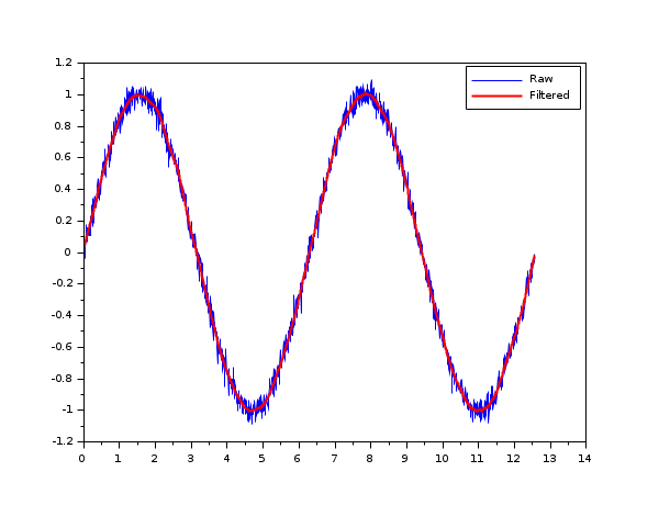
The sgolay function can be used to construct FIR filter with no group delay. The following instructions explains what the sgolayfilt function does:
dt = 0.01;
t = (0:0.01:4*%pi)';
x = sin(t)+0.05*rand(t,'normal');

nf = 61;
[B,C] = sgolay(3,nf);
nfs2 = floor(nf/2);

//compute the middle part of the filtered signal
xfm = filter(B(nfs2+1,:), 1, x);
xfm = xfm(nf:$);
//compute the left part of the filtered signal
xfl = B(1:nfs2,:)*x(1:nf);
//compute the right part of the filtered signal
xfr = B(nfs2+2:nf,:)*x($-nf+1:$);
clf
plot(t,x,'b',t,[xfl;xfm;xfr],'r');
gce().children(1).thickness = 2;
legend(["Raw","Filtered"]);
The above script generate this graph:
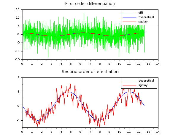
It can also be used to obtain approximate derivatives:
dt=0.01;
t = (0:0.01:4*%pi)';
x = sin(t)+0.03*rand(t,'normal');

nf = 61;
[B,C] = sgolay(3,nf);
nfs2 = floor(nf/2);

dx=-conv(x,C(:,2)',"valid");
d2x=2*conv(x,C(:,3)',"valid");

clf();
subplot(211)
plot(t(2:$),diff(x)/dt,'g',t,cos(t),'b',t(nfs2+1:$-nfs2),dx/dt,'r');
legend(["diff","theoretical","sgolay"]);
title("First order differentiation")
subplot(212)
plot(t,-sin(t),'b',t(nfs2+1:$-nfs2),d2x/(dt^2),'r');
legend(["theoretical","sgolay"]);
title("Second order differentiation")
Bibliography
Abraham Savitzky et Marcel J. E. Golay, « Smoothing and Differentiation of Data by Simplified Least Squares Procedures », Analytical Chemistry, vol. 8, no 36, 1964, p. 1627–1639 (DOI 10.1021/ac60214a047)
See Also
- sgolayfilt — Filter signal using Savitzky-Golay Filter.
- conv — discrete 1-D convolution.
History
| Version | Description |
| 6.1.1 | Function added. Courtesy of Serge Steer, INRIA |
| Report an issue | ||
| << remezb | Filters | sgolaydiff >> |