lqi

Linear quadratic integral compensator (full state)

Syntax

[K, X] = lqi(P, Q, R)
[K, X] = lqi(P, Q, R, S)

Arguments

P: The plant state space representation (see syslin) with nx states, nu inputs and ny outputs.
Q: Real nx+ny by nx+ny symmetric matrix,
R: full rank nu by nu real symmetric matrix
S: real nx+ny by nu matrix, the default value is zeros(nx+ny,nu)
K: a real matrix, the optimal gain
X: a real symmetric matrix, the stabilizing solution of the Riccati equation

Description

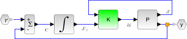
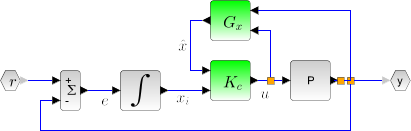
This function computes the linear quadratic integral full-state gain K for the plant P. The associated system block diagram is:

The plant P is given by its state space representation

$\text{P}=\left\lbrace \begin{array}{l}\dot{x}=A x+B u\\y=C x+D u \end{array}\right. \text{ in continuous time or } \text{P}=\left\lbrace \begin{array}{l}\overset{+}{x}=A x+B_2 u\\y=C x+D u \end{array}\right. \text{ in discrete time.}$

The cost function in l2-norm is:

$\int_{t=0}^\infty{z(t)$

$\sum_{k=0}^\infty{z(k)$

where $z=\left[\begin{array}{l}x\\x_i \end{array}\right]$ and x_i is the integrator(s) state(s);

It is assumed that matrix R is non singular.

If the full state of the system is not available, an estimator of the plant state can be built using the lqe() function.

Algorithm

The lqi function solves the lqr problem for the augmented plant

$\left\lbrace \begin{array}{l}\left[\begin{array}{l}\dot{x}\\ \dot{x_i} \end{array}\right]=\left[\begin{array}{ll}A&0\\-C&0 \end{array}\right]\left[\begin{array}{l}x\\x_i \end{array}\right]+\left[\begin{array}{l}B\\-G \end{array}\right] u \end{array}\right. \text{ in continuous time }$

$\text{P}=\left\lbrace\begin{array}{l}\left[\begin{array}{l}\overset{+}{x}\\ \overset{+}{x_i} \end{array}\right]=\left[\begin{array}{ll}A&0\\-C dt&I \end{array}\right]\left[\begin{array}{l}x\\x_i \end{array}\right]+\left[\begin{array}{l}B\\-G dt \end{array}\right] u \end{array} \right.\text{ in discrete time }$

Examples

Linear quadratic integral controller of a simplified disk drive using state observer.

//Disk drive model
G=syslin("c",[0,32;-31.25,-0.4],[0;2.236068],[0.0698771,0]);
t=linspace(0,20,2000);
y=csim("step",t,G);

//State estimator
Wy=1;
Wu=1;
S=0;
Q=G.B*Wu*G.B';
R=Wy+G.D*S + S'*G.D+G.D*Wu*G.D';
S=G.B*Wu*G.D'+S;

//State estimator
[Kf,X]=lqe(G,Q,R,S);
Gx=observer(G,Kf);

//LQI compensator

wy=100;
Q= wy*blockdiag(G.C'*G.C,1);
R=1/wy;
Kc=lqi(G,Q,R);
//full controller
K=lft([1;1]*(-Kc(1:2)*Gx(:,[2 1])+Kc(3)*[1/%s 0]),1);//e-->u

//Full system
H=(-K*G)/.(1);// full system transfer function

y=csim("step",t,H);
clf;plot(t,y)

History

Version	Description
6.0	lqi() function introduced.

Report an issue
<< lqg_ltr	Linear Quadratic	lqr >>

Copyright (c) 2022-2024 (Dassault Systèmes)
Copyright (c) 2017-2022 (ESI Group)
Copyright (c) 2011-2017 (Scilab Enterprises)
Copyright (c) 1989-2012 (INRIA)
Copyright (c) 1989-2007 (ENPC)
with contributors

Last updated:
Mon Mar 27 11:52:43 GMT 2023

lqi