Please note that the recommended version of Scilab is 2026.0.1. This page might be outdated.
See the recommended documentation of this function
fsolve
find a zero of a system of n nonlinear functions
Syntax
[x [,v [,info]]]=fsolve(x0,fct [,fjac] [,tol])
Arguments
- x0
real vector (initial value of function argument).
- fct
external (i.e function or list or string).
- fjac
external (i.e function or list or string).
- tol
real scalar. precision tolerance: termination occurs when the algorithm estimates that the relative error between x and the solution is at most tol. (
tol=1.d-10is the default value).- x :
real vector (final value of function argument, estimated zero).
- v :
real vector (value of function at x).
- info
termination indicator
- 0
improper input parameters.
- 1
algorithm estimates that the relative error between x and the solution is at most tol.
- 2
number of calls to fcn reached
- 3
tol is too small. No further improvement in the approximate solution x is possible.
- 4
iteration is not making good progress.
Description
find a zero of a system of n nonlinear functions in n variables by a modification of the powell hybrid method. Jacobian may be provided.
0 = fct(x) w.r.t x.
fct is an "external". This external returns
v=fct(x) given x.
The simplest syntax for fct is:
[v]=fct(x).
If fct is a character string, it refers to a C or
Fortran routine which must be linked to Scilab. Fortran calling sequence
must be
fct(n,x,v,iflag)
integer n,iflag
double precision x(n),v(n)
and C Syntax must be
Incremental link is possible (help link).
jac is an "external". This external returns
v=d(fct)/dx (x) given x.
The simplest syntax for jac is:
[v]=jac(x).
If jac is a character string, it refers to a to a
C or Fortran routine which must be linked to Scilab calling sequences are
the same as those for fct. Note however that v must be a nxn array.
Examples
// A simple example with fsolve
a=[1,7;2,8];
b=[10;11];

function y=fsol1(x)
  y=a*x+b
endfunction
function y=fsolj1(x)
  y=a
endfunction

[xres]=fsolve([100;100],fsol1);
a*xres+b

[xres]=fsolve([100;100],fsol1,fsolj1);
a*xres+b

// See SCI/modules/optimization/sci_gateway/fortran/Ex-fsolve.f
[xres]=fsolve([100;100],'fsol1','fsolj1',1.e-7);
a*xres+b
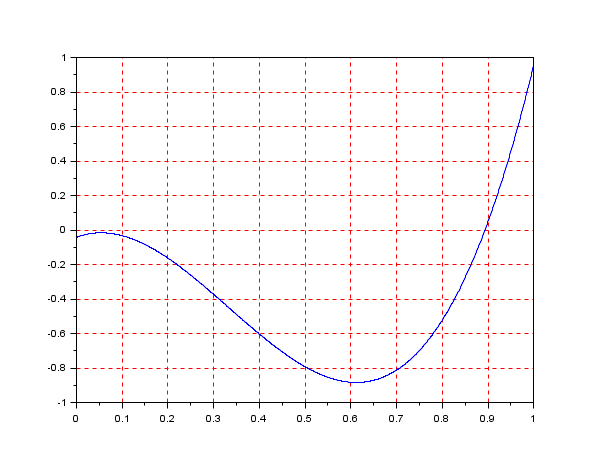
For some starting points and some equations system, the fsolve method can fail. The fsolve method is a local search method. So, to have a good chance to find a solution to your equations system, you must ship, a good starting point to fsolve.
Here is an example on which fsolve can fail:
// Another example with fsolve
function F=feuler(x, r)
  F=x-r-dt*(x.^2-x.^3);
endfunction
function J=dFdx(x)  //Definition of the Jacobian
   J=1-dt*(2*x-3*x^2);
endfunction

r = 0.04257794928862307 ;
dt = 10;

[x,v,info]=fsolve(r,list(feuler,r),dFdx); // fsolve do not find the solution
disp(v); // The residual
disp(info); // The termination indicator

[x,v,info]=fsolve(1,list(feuler,r),dFdx); // fsolve find the solution
disp(v); // The residual
disp(info); // The termination indicator

clf();
x=linspace(0,1,1000);
plot(x,feuler(x))
a=gca();
a.grid=[5 5];

So, each time you use fsolve, be sure to check the termination indicator and the residual value to see if fsolve has converged.
See also
| Report an issue | ||
| << NDcost | Optimization and Simulation | karmarkar >> |