Solution output (ODE and DAE solvers)
Specialized output of solvers
Syntax
sol = solver(..., options)
solext = solver(sol, tfinal, options)
y = sol(t)
[y,yd] = sol(t)
... = sol(t,i)
Arguments
| sol, solext | MList of |
| tfinal | final time of extended solution |
| options | a sequence of optional named arguments (see sundials options) |
| t | a vector of time values |
| y,yd | The matrices of interpolated solution and its derivative at times values given in t |
| i | the component of the solution to interpolate. If the state of the equation is not a vector then i indexes the state as a flatened vector. |
Description
When a solution has to be further evaluated at arbitrary points which are not known in advance, then the syntax
sol = solver(..., options)
yields a MList with fields:
| solver | the solver name, "arkode", "cvode" or "ida" | ||||||||||||||||||||||||||||
| method | the name of the method used by the solver. For example cvode can use "ADAMS" or "BDF", ida uses only "BDF" and the list of arkode methods is given in its dedicated help page. | ||||||||||||||||||||||||||||
| interpolation | a string giving the interpolation method used by the solver to compute the solution between solver steps. The solvers arkode and cvode interpolation is based on the basis vectors used by the solver and thus the interpolation method is denoted "native". arkode can use Hermite or Lagrange interpolation and the polynomial degree can be chosen when calling the solver, hence the string is "Hermite(p)" or "Lagrange(p)" where p is the actual degree. | ||||||||||||||||||||||||||||
| linearSolver | the linear solver used by the method, if applicable. Can be "none" when using the Adams method with cvode or an explicit method with arkode. When using an implicit method relying on Newton method for the iterations, and when the linear solver is matrix based, i.e. implements a direct method, this string can be "dense", "band" or "sparse" depending on the format of the Jacobian provided by the user. | ||||||||||||||||||||||||||||
| nonLinearSolver | the nonlinear solver used by the method, which can be "none" for explicit methods, "fixedPoint" when functional iterations are used or "Newton", when the Newton method is used, both when using an implicit method (e.g. BDF or any DIRK method). | ||||||||||||||||||||||||||||
| rtol,atol | the relative and absolute tolerance used by the solver to achieve adaptive time stepping. | ||||||||||||||||||||||||||||
| t,y,yp | vector of time points used by the solver and solution at time points (yp is defined when using ida) | ||||||||||||||||||||||||||||
| te,ye,ype,ie | time of event, solution and index of event | ||||||||||||||||||||||||||||
| manager | pointer to the internal OdeManager object | ||||||||||||||||||||||||||||
| stats | a structure gathering the solver statistics:
|
Solution interpolation and extension
For an arbitrary time vector t, with values in the interval [t0,tf] the following syntax
y = sol(t)
[y,yd] = sol(t)
... = sol(t,i)
yields by costless interpolation in y and yd the same approximation as if components of t where used in the
tspan argument in the solver call.
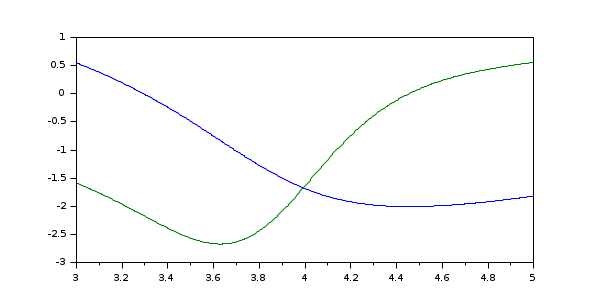
The derivative of solution can also be obtained with [y,yd]=sol(t) and a particular component
i of the solution is obtained with y=sol(t,i). For example, the solution of the Van Der Pol
equation can be refined in [3,5] with the following code:
The syntax
solext = solver(sol, tfinal, options)
extends the solution by restarting the solver from
initial time sol.t($) and initial condition sol.y(:,$) (you cannot
use a different solver or the same solver with a different method).
This extension can be typically used when you know in advance that the solution is not differentiable at some
time point. By stopping then restarting the solver at time of discontinuity you optimize solver effort by
avoiding very small time steps.
In the options sequence you can change almost all (but not the solver method) previously used options used in the call
of the solver which yielded sol. The right hand side or the residual function and the initial conditions can be overriden
by using the specific rhs, res, y0 or yp0 options, respectively.
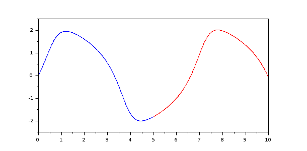
Here is an example where we extend the solution of the Van Der Pol equation:
sol = arkode(%SUN_vdp1, [0 5], [0; 2]);
solext = arkode(sol, 10);
t = linspace(0,5,500);
plot(t,sol(t,1))
t = linspace(5,10,500);
plot(t,solext(t,1),'r')
See also
- arkode — SUNDIALS ordinary differential equation additive Runge-Kutta solver
- cvode — SUNDIALS ordinary differential equation solver
- ida — SUNDIALS differential-algebraic equation solver
- User functions — Coding user functions used by SUNDIALS solvers
- Options (ODE and DAE solvers) — Changing the default behavior of solver
| Report an issue | ||
| << Sensitivity (ODE) | Options, features and user functions | User functions >> |