ida
SUNDIALS differential-algebraic equation solver
Syntax
[t,y] = ida(F,tspan,y0,yp0,options)
[t,y,info] = ida(F,tspan,y0,yp0,options)
sol = ida(...)
solext = ida(sol,tfinal,options)
ida(...)
Arguments
| F | a function, a string or a list, the residual of the differential-algebraic equation |
| tspan | double vector, time interval or time points |
| y0,yp0 | double arrays: initial state and initial state derivative |
| options | a sequence of optional named arguments, see the solvers options |
| t | vector of time points used by the solver |
| y | array of solution at time values in t |
| sol, solext | MList of |
| info | MList of |
| tfinal | final time of extended solution |
Description
ida computes the solution of real or complex ordinary different-algebraic equation defined by

It is an interface to the ida solver of SUNDIALS library using BDF method. The simplest call of ida is when tspan is a two component vector:
It is an interface to the idas solver of SUNDIALS library using BDF method. The solver has a specific feature which allows to compute the sensitivity with respect to a vector of parameters present in the initial conditions and/or the residual equation (see the DAE Sensitivity help page). The simplest call takes the form
[t,y] = ida(F,[t0 tf],y0,yp0)
[t,y,info] = ida(F,[t0 tf],y0,yp0)
where F(t,y,y') is the right hand side usually called "residual" of the DAE, t0, tf are the initial and final time, y is the
array of solution [y(t(1)),y(t(2)),...] at time values in t, info.yp is the
array of solution derivative [y'(t(1)),y'(t(2)),...]. Concatenation is done on next dimension if
y0 is not a column vector. The time values in t
are those used by the solver to meet default relative and absolute estimated local error (which can be changed in options).
In the simplest case the DAE residual is computed by a Scilab function with three arguments, for example for  F is coded as
function res=F(t, y, yp)
  res = yp+y
end
See the User functions help page to learn how to pass extra parameters and/or use DLL entrypoints. When t has more than two components:
[t,y] = ida(F,[t0 t1 ... tf],y0,yp0)
[t,y,info] = ida(F,[t0 t1 ... tf],y0,yp0)
the solution is computed at prescribed points with the same precision as the two components syntax. However, the result may slightly differ (within chosen tolerance) since t1-t0 may give a different guess of the initial step used by the solver. Provided that the initial step is the same, further solver internal steps
will be the same and solution at intermediate user points is computed by continuous extension formulas.
When searching for  where some functions defined in
 options vanish (see the Events help page) the syntax
[t,y,info] = ida(F,tspan,y0,yp0,options)
allows to recover  values in
 info.te, info.ye, info.ype and in info.ie the number(s) of the vanishing function.
When solution has to be further evaluated at arbitrary points which are not known in advance, then the syntax
sol = ida(F,[t0 tf],y0,yp0)
yields an MList of _odeSolution type, which can be used later as an interpolant, see the solution output help page.
When y0 and/or yp0 do not fullfill the equation at initial time they can be used as initial guesses when using the calcIc option,
see the Initial conditions section.
When no ouput argument is given, the only way to have access to the solution at solver or user time steps is to use a user callback (see the SUNDIALS user functions help page). For example, when there could be memory issues (e.g. if the dimension of the solution vector is very large) this allows to write the solution to disk.
Example
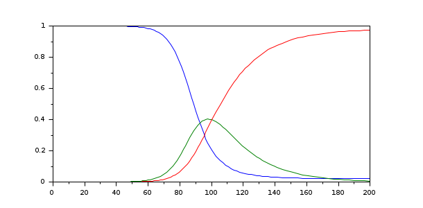
In the following example, we solve the equations of the SIR model. The DAE residual is computed by the function %SUN_sir (defined in the SUNDIALS module):
function r=%SUN_sir(t, y, yp)
    r = [yp(1)+0.2*y(1)*y(2)
         yp(2)-0.2*y(1)*y(2)+0.05*y(2)
          y(1)+y(2)+y(3)-1];
end
y0  = [1-1e-6; 1e-6; 0];
yp0 = [-2e-7; 1.5e-7; 5e-8];
[t,y] = ida(%SUN_sir, [0,200], y0, yp0);
clf
plot(t, y)
Initial conditions
When y(0) is known but y'(0) is not known it can be computed by using the calcIc option with value "y0yp0"
and yp0 is used as an initial guess:
y0  = [1-1e-6; 1e-6; 0];
yp0 = zeros(3,1);
[t,y,info] = ida(%SUN_sir, [0,200], y0, yp0, calcIc="y0yp0");
disp(info.yp(:,1))
When the DAE is semi-explicit and of index one, this option also allows to compute purely algebraic states
by using the yIsAlgebraic = idx option, where idx is a vector with
the indexes of such states. When y'(0) is known but y(0) is not, use calcIc option with value "y0".
When the DAE is of index two or more these options should not be used and coherent initial conditions must be given for all states, and
setting the option suppressAlg is recommended (see below).
DAE with high index
When the DAE is of high index, the suppressAlg option can help the solver effort.
If suppressAlg = %T then the algebraic variables (given with the yIsAlgebraic option)
are excluded from the local error test. The use of this option (with %T value) is discouraged when solving DAE systems of index one
whereas it is often the only way to obtain a solution for systems of index two or more. See the following example below (a circular pendulum DAE of index two).
function out=res(t, y, yd)
    x=y(1:2);
    xd=yd(1:2);
    u=y(3:4);
    ud=yd(3:4);
    lambda=y(5);
    out=[xd-u
         ud+x*lambda+[0;1]
         x'*u];
end

// One period
T = 7.4162987092054876;
y0=[1;0;0;0;0];
yd0=[0;0;0;-1;0];
[t,y]=ida(res,T,y0,yd0,t0=0,yIsAlgebraic=5,suppressAlg=%t)
See also
- arkode — SUNDIALS ordinary differential equation additive Runge-Kutta solver
- cvode — SUNDIALS ordinary differential equation solver
- User functions — Coding user functions used by SUNDIALS solvers
- Options (ODE and DAE solvers) — Changing the default behavior of solver
Bibliography
A. C. Hindmarsh, P. N. Brown, K. E. Grant, S. L. Lee, R. Serban, D. E. Shumaker, and C. S. Woodward, "SUNDIALS: Suite of Nonlinear and Differential/Algebraic Equation Solvers," ACM Transactions on Mathematical Software, 31(3), pp. 363-396, 2005. Also available as LLNL technical report UCRL-JP-200037.
Alan C. Hindmarsh, Radu Serban, Cody J. Balos, David J. Gardner, Daniel R. Reynolds, and Carol S. Woodward, "User Documentation for ida", 2021, v6.1.1, available online at https://sundials.readthedocs.io/en/latest/ida.
| Report an issue | ||
| << cvode | SUite of Nonlinear and DIfferential/ALgebraic equation - SUNDIALS solvers | kinsol >> |