Options (ODE and DAE solvers)
Changing the default behavior of solver
Syntax
... = arkode( ... , options)
... = cvode( ... , options)
... = ida( ... , options)
Common options
The default behavior of the solver can be tuned by specifying a sequence of named parameter values. These parameters are the following:
| options | A struct with options field names and corresponding values. Specifying the options with a struct allows to use the same options set in different solver calls. Values are overriden by separately setting individual options. |
| method | The solver method given as a string. cvode accepts "ADAMS" or "BDF", ida accepts only "BDF" and the table of arkode methods is given in a dedicated section. |
| linearSolver, linSolMaxIters, precType, precBand | These options allow to specify the linear solver. Please see the dedicated linear solvers page. |
| nonLinSol, nonLinSolMaxIters, nonLinSolAccel | nonLinSol precises the method to use in non-linear iterations when using an implicit solver method, "Newton" (the default) or "fixedPoint". The maximum number of non-linear iterations is given by nonLinSolMaxIters and nonLinSolAccel gives the number of acceleration Anderson vectors in fixed point iterations. |
| t0 | When the time span given to the solver is a scalar, it is considered as the final time and the initial time is undetermined. The t0 option allows to specify the initial time in that case. |
| rhs, res | These options allow to change the right hand side function (when using cvode or arkode) or the residual function (when using ida) when extending a solution. |
| y0, yp0 | These options allow to change the initial condition of the solution (and its derivative when using ida) when extending a solution. |
| rtol | The scalar relative tolerance to control the local error estimator (default value is 1e-4). |
| atol | The absolute tolerance controlling the local error. It can be a scalar or an array of the same dimension as the differential equation state (default value is 1e-6). Note that unlike rtol, atol should take into account the scale of the solution components. |
| ratol | The absolute tolerance controlling the residual in nonlinear iterations. Can be a scalar or an array of the same dimension as the differential equation state. |
| maxOrder | Allows to bound the maximum order of the method. The default maximum order of the method is 5 for the BDF method and 12 for the ADAMS method and any lower value can be chosen. This option is not available when using arkode. |
| h0 | Proposed initial step. By default the solver computes the initial step by estimating second derivatives. |
| hMin | Minimum value of solver time steps. Can make convergence fail if chosen too large. |
| hMax | Maximum value of solver time steps. Use it with care and only if the solver misses an event
(for example a discontinuity) because of a large step. If you need a finer discretization of time
span don't use an interval as time span but a vector like |
| maxSteps | Maximum solver internal steps between user steps. You may have to increase the default value (500) when
the integration interval is large and a small number of user
time steps have been specified in |
| refine | The number of complimentary time points added between two successive solver time points by using the current
interpolation method (depending on the solver).
This option is active when using an interval function acc=bounce(t, y, g) acc = [y(2); -g] endfunction function [out, term, dir]=bounce_ev(t, y) out = y(1); term = 1; dir = -1; endfunction [t,y] = cvode(list(bounce,9.81), [0 10], [1;0], events=bounce_ev); [tr,yr] = cvode(list(bounce,9.81), [0 10], [1;0], events=bounce_ev,refine=4); plot(tr,yr(1,:),'-o',t,y(1,:),'or') legend("refined","original"); 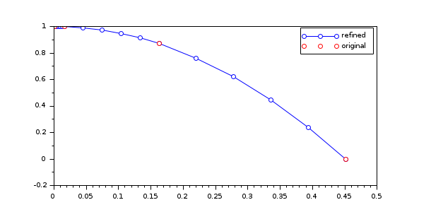 |
| negative, nonPositive, nonNegative, positive, | A vector with the indices of the solution to constrain. When a component of the theoretical solution has a constant sign then any of the following four constraints can be imposed: yi<0, yi<=0, y>=0, yi>0. Solver steps are eventually reduced to verify the constraint but repeated failures may indicate that the step tolerance has to be changed (see rtol and atol options). See the following classical problem, where reducing the maximum step is not enough to catch the "knee": tspan = [0 2]; y0 = 1; deff("yd=odefcn(t,y)","yd=((1-t)*y - y^2)/1e-6"); [t1,y1] = cvode(odefcn, tspan, y0, method="BDF", hMax = 0.2); [t2,y2] = cvode(odefcn, tspan, y0, method="BDF", hMax = 0.2, nonNegative=1); plot(t1,y1,"-o",t2,y2,"-or"); legend("No constraint","nonNegative"); 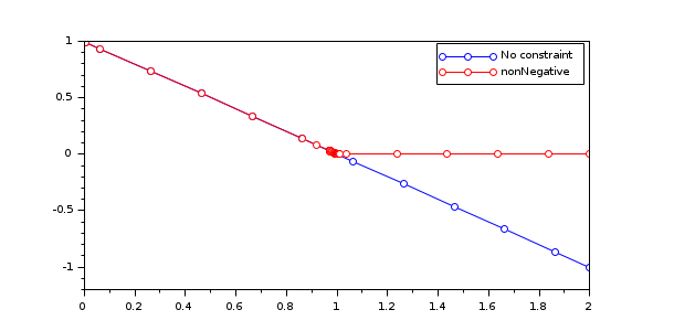 |
| jacobian, jacBand, jacPattern, jacNonZeros | These options allow to specify a user-supplied Jacobian or its approximation when an implicit method is used. Please see the dedicated Jacobian page. |
| events, nbEvents, evDir, evTerm | The solver can record the values of (t,y) when a component of a given function g(t,y) vanishes. A detailed explanation and examples are given in the dedicated Events page. |
| callback | The solver can call a user function after each successfull internal or user prescribed step. See the dedicated Callback page for explanations and use cases. |
| nbThreads | A positive integer. This option is available when Scilab has been compiled with OpemMP support (https://www.openmp.org). It allows the use of multiple cores of the processor during calculations involving vectors in the solver algorithm. However, testing has shown that vectors should be of length at least 100000 before the overhead associated with creating and using the threads is made up by the parallelism in the vector calculations. Moreover, in order to fully take advantage of this option, C or C++ entrypoints should also be used. |
cvode and ida options
cvode and ida accept the following specific options related to pure quadrature states and sensitivity computation:
| quadRhs, yQ0 | See the specific pure quarature help page. |
| sensPar, sensParIndex, sensRhs, sensRes, sensErrCon, sensCorrStep, typicalPar, yS0, ypS0 | These options allow to trigger and parametrize sensitivity computation. Please see the dedicated ODE Sensitivity and DAE Sensitivity help pages. |
cvode options
cvode accept the following specific options:
| projection, projectError | See the projection section of the cvode help page. |
ida options
ida accepts options that only make sense for differential-algebraic implicit equations:
| calcIC | A string specifying the type of initial condition to compute if |
| yIsAlgebraic | A vector of integer indices of algebraic states. |
| supressAlg | A boolean. If suppressAlg = %T, then the algebraic variables are excluded from the local error test. See the dedicated section in the ida help page. |
arkode options
arkode accepts the following specific options:
| stiffRhs | A function, a string or a list, the stiff right hand side of the differential equation when implicit/explicit integration is to be performed. See the paragraph about implicit/explicit solver splitting in the arkode help page. |
| ERKButcherTab, DIRKButcherTab | A matrix of size (s+2,s+1) or (s+1,s+1) where s is the number of stages of the method. See the paragraph about custom tableaux in the arkode help page. |
| fixedStep | A positive number giving the fixed step value when adaptive stepping is to be disabled. Be warned that with a fixed step no error control occurs hence the computed solution may be very inaccurate. |
| mass | A Scilab function, a list, a string or a matrix (dense or sparse). When passed as a constant matrix or as the output of a Scilab function, the mass matrix can be a dense, sparse or band matrix. In the latter case
the See the Mass section on the arkode help page for more information and examples. |
| massBand | A vector of two positive integers [mu,ml] giving respectively the upper and lower half bandwidth of the mass matrix. |
| massNonZeros | An integer, the number of non-zeros terms when the Mass matrix is sparse and given as the output of a SUNDIALS DLL entrypoint. |
| interpolation | The interpolation method used to compute the solution between solver steps when dense output is required. "Hermite" (the default) and "Lagrange" interpolation methods can be chosen when using arkode. The Lagrange method is recommended when the ode is stiff and the rhs has a large Lipschitz constant. |
| degree | The degree of the polynomial used by arkode for dense output. Defaults to 3 for both Hermite (maximum is 5) and Lagrange methods (maximum is 3). |
See also
- arkode — SUNDIALS ordinary differential equation additive Runge-Kutta solver
- cvode — SUNDIALS ordinary differential equation solver
- ida — SUNDIALS differential-algebraic equation solver
- User functions — Coding user functions used by SUNDIALS solvers
| Report an issue | ||
| << SUNDIALS Linear Solvers | Options, features and user functions | Pure quadrature >> |