plot2d
2D plot
Syntax
plot2d()   // example
plot2d(y)
plot2d(x, y)
plot2d(logflag, x, y)
plot2d(.., y, style)
plot2d(.., y, style, strf)
plot2d(.., y, style, strf, leg)
plot2d(.., y, style, strf, leg, rect)
plot2d(.., y, style, strf, leg, rect, nax)
plot2d(.., y, key1=value1, key2=value2, ..)
hdl = plot2d(...)
Arguments
- x
a real matrix or vector of abscissae. If omitted, abscissae are assumed to be
1:nfor all curves, wherenis the number of points in curves, as given byy.- y
real matrix or vector: Ordinates
- key1=value1, key2=value2, ...
The following options
logflag,style,strf,leg,rect,nax,frameflag, andaxesflagdescribed below can either be listed in the right order as listed in the synopses, or provided in any order afteryas named arguments, for instance like inplot(y, frameflag=3, leg="Curve 1@Curve 2").- logflag
Sets the linear or logarithmic scale for both X and Y axes. Possible values are
"nn","nl","ln"or"ll"."n"stands for normal scale ;"l"stands for logarithmic. The first letter set the X axis. The second one sets the Y axis.- style
Sets the respective line or mark styles of the curves. It is a vector of decimal integers with one element per curve:
if
style(i)is strictly positive, the curve is drawn as plain line andstyle(i)defines the index of the color used to draw the curve (see getcolor).if
style(i)is negative or zero, the given curve points are drawn using marks. Thenabs(style(i))is the mark's id.
Note that all curves properties -- like also their color, thickness, marks colors, etc -- can be set through their handles (see polyline_properties).
- strf
3-character-long string
"abc"specifying all together if legends must be displayed, and the values offrameflagandaxesflag. By default,strf= "081". "a", "b" and "c" are:a : controls the display of captions:
a=0 : no caption. a=1 : captions given by the optional argument legare displayed.b : frameflaginteger code in [0,9], controlling the computation the actual coordinate ranges, as described below.c : axesflaginteger code in [0:5 9], controlling the display and position of X and Y axes, as described below.- leg
Single string
"leg1@leg2@...."setting the legends leg1, leg2, etc for the respective curves #1, #2, etc. The default is" ". The block of legends is drawn on the bottom, below the x-axis.After plotting, the handle of the block of legends can be retrieved with
gca().children(2). legend or legends can also be used instead ofleg.- rect
Vector of decimal numbers
[xmin, ymin, xmax, ymax]setting the minimal bounds requested for the plot.[xmin, xmax]is the X-axis range, and[ymin, ymax]is the Y-axis one.This argument works with the
frameflagoption to specify how the actual axes boundaries are computed. If theframeflagoption is not given, it is supposed to beframeflag=7.The axes boundaries can also be customized through the
gca().data_boundsproperty of the axes (see axes_properties).- nax
Vector of decimal integers
[nx,Nx,ny,Ny]specifying the numbers Nx and Ny of major ticks, and the numbers nx and ny of minor ticks between 2 majors, for both respective axes. To use autoticking on an axis, set Nx=-1 or Ny=-1.If the
axesflagoption is not specified, usingnaxsets and usesaxesflag=9.- frameflag
controls the computation of the actual coordinate ranges from the minimal requested values. The associated value should be an integer ranging from 0 to 8.
frameflag axes bounds other actions 0 unchanged 1 from rect 2 from input x,y 3 from rect isometric axes 4 from input x,y isometric axes 5 from rect pretty axes 6 from input x,y pretty axes 7 from rect all replot with new scales 8 from input x,y all replot with new scales 9 from input x,y Pretty axes. All replot with new scales The setting of axes boundaries can also be customized through the
gca().data_bounds,gca().tight_limits,gca().data_bounds, andgca().isoviewproperties (see axes_properties).- axesflag
integer code in [0:5 9], controlling the display and position of X and Y axes.
The axes aspect can also be customized directly through the
gca().box,gca().axes_visible,gca().x_location, andgca().y_location, properties (see axes_properties).axesFlag .box .axes_visible axes position comments 0 "off" ["off" "off"] Naked plot 1 "on" ["on" "on"] 2 "on" ["off" "off"] Naked box 3 "off" ["on" "on"] y_location="right" 4 "off" ["on" "on"] crossed @ middle 5 "on" ["on" "on"] crossed @ middle 9 "off" ["on" "on"] (default setting) - hdl
This optional output is a vector containing the handles of the created
Polylineentities. Usehdlto modify properties of a specific or all entities after they are created. For a list of properties, see polyline_properties.
Description
plot2d plots a set of 2D curves. Piecewise linear interpolation
is done between the given curve points.
Any point with y(i)=Nan is masked: no mark and no segment to its
neighboors are displayed.
For any point with y(i)=±Inf, a vertical segment starting
from each of its both neighboors is drawn in the ± direction, up to the current ceil
or down to the current floor of the axes.
By default, successive calls to plot2d() overplots new curves over existing ones.
Autoclearing for each new plot can be set using gca().auto_clear="on".
Please see axes properties.
clf can also be used to manually clear
the whole figure.
If you are familiar with Matlab plot syntax, you should use
plot instead.
If x and y are vectors,
plot2d(x,y,…) plots vector y versus
vector x. x and y
vectors should have the same number of entries.
If x is a vector and y a
matrix plot2d(x,y,…) plots each columns of
y versus vector x. The
number of rows of y must be equal to the number of
x entries.
If x and y are matrices,
plot2d(x,y,…) plots each columns of y
versus corresponding column of x.
x and y must then have the same sizes.
If y is a vector, plot2d(y,…)
plots vector y versus vector
1:size(y,'*').
If y is a matrix, plot2d(y,…)
plots each columns of y versus vector
1:size(y,1).
Enter the command plot2d() to see a demo.
Other high level plot2d functions exist:
plot2d2 same as
plot2dbut the curve is supposed to be piecewise constant.plot2d3 same as
plot2dbut the curve is plotted with vertical bars.plot2d4 same as
plot2dbut the curve is plotted with vertical arrows.
Examples
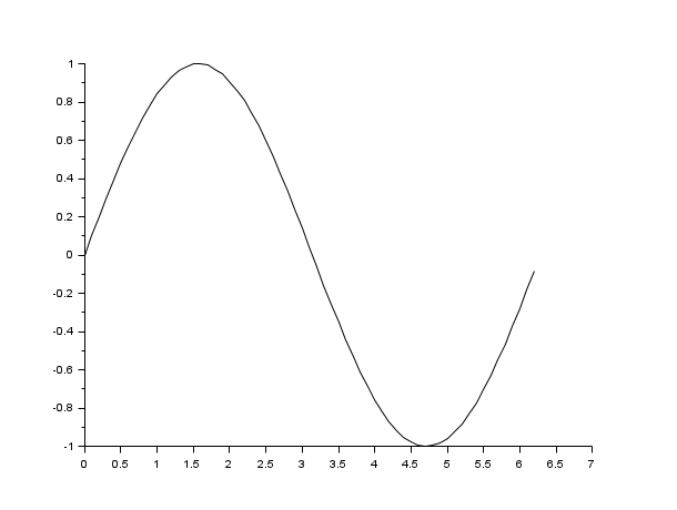
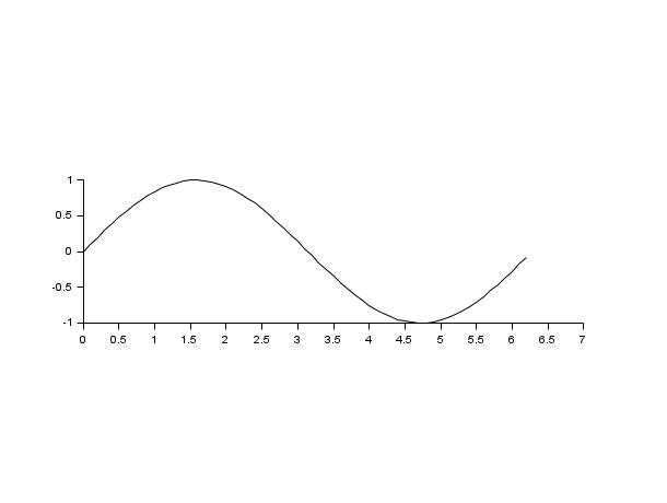
// x initialisation
x=[0:0.1:2*%pi]';
//simple plot
plot2d(sin(x));

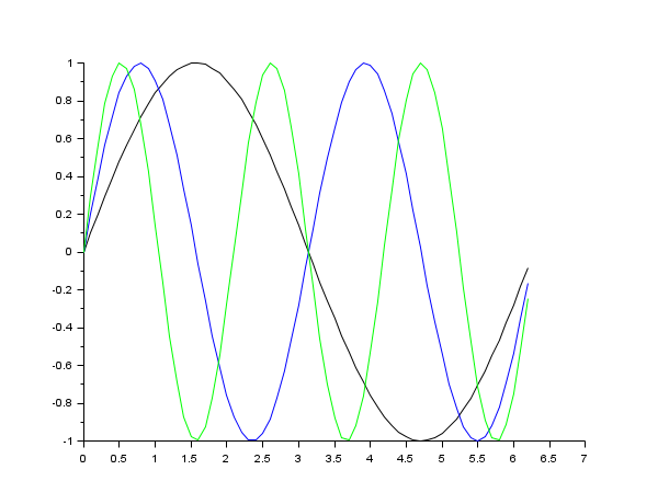
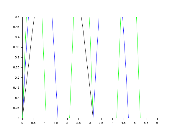
// multiple plot giving the dimensions of the frame
clf();
x=[0:0.1:2*%pi]';
plot2d(x,[sin(x) sin(2*x) sin(3*x)],rect=[0,0,6,0.5]);
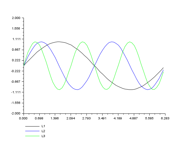
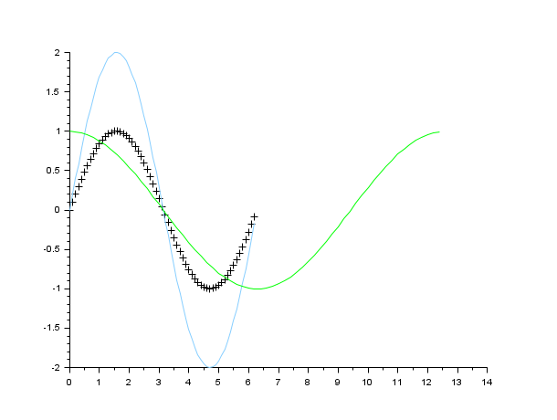
//multiple plot with captions and given tics + style
clf();
x=[0:0.1:2*%pi]';
plot2d(x,[sin(x) sin(2*x) sin(3*x)],..
       [1,2,3],leg="L1@L2@L3",nax=[2,10,2,10],rect=[0,-2,2*%pi,2]);

// auto scaling with previous plots + style
clf();
x=[0:0.1:2*%pi]';
plot2d(x,sin(x),-1);
plot2d(x,2*sin(x),12);
plot2d(2*x,cos(x),3);
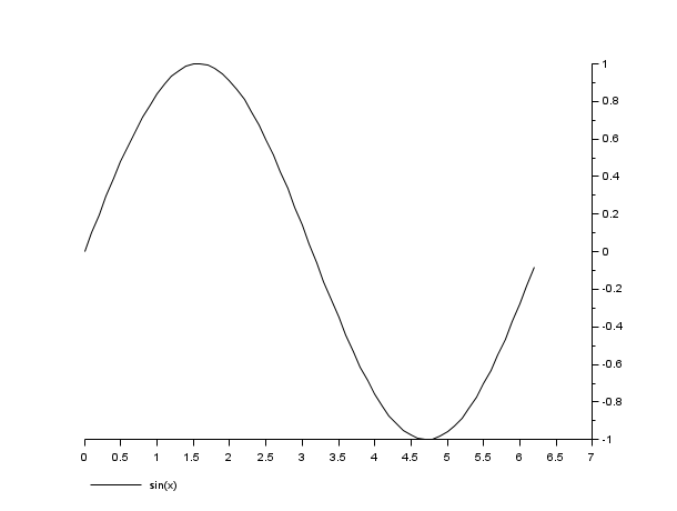
// axis on the right
clf();
x=[0:0.1:2*%pi]';
plot2d(x,sin(x),leg="sin(x)");
a=gca(); // Handle on axes entity
a.y_location ="right";
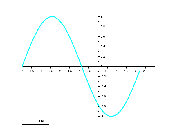
// axis centered at (0,0)
clf();
x = [0:0.1:2*%pi]';
poly1 = plot2d(x-4,sin(x),1,leg="sin(x)");
a = gca(); // Handle on axes entity
a.x_location = "origin";
a.y_location = "origin";
// Some operations on entities created by plot2d ...
isoview()
a = gca();
poly1.foreground = 4; // another way to change the style...
poly1.thickness = 3;  // ...and the thickness of a curve.
poly1.clip_state='off'; // clipping control
// find the legend
leg = findobj(gca(),"type","Legend");
leg.font_style = 9;
leg.line_mode = "on";
isoview("off")
See also
- plot — 2D plot
- .polyline_style — description of the Polyline entity properties
- plot2d2 — 2D plot (step function)
- plot2d3 — 2D plot (vertical bars)
- plot2d4 — 2D plot (arrows style)
- polarplot — Plot polar coordinates
- gca — Return handle of current axes.
- close — Closes graphic figures, progression or wait bars, the help browser, xcos, the variables browser or editor.
- axes_properties — description of the axes entity properties
- clf — Clears and resets a figure or a frame uicontrol
History
| Version | Description |
| 2025.0.0 | Function returns the created handle(s). |
| Report an issue | ||
| << plot | 2d_plot | plot2d2 >> |