Please note that the recommended version of Scilab is 2026.1.0. This page might be outdated.
See the recommended documentation of this function
ellipj
Jacobi elliptic functions
Syntax
sn = ellipj(x, m)
[sn, cn] = ellipj(x, m)
[sn, cn, dn] = ellipj(x, m)
struc = ellipj(funames, x, m)
Arguments
- x
- Array of real or complex numbers inside the fundamental rectangle defined by the elliptic integral.
- m
- Scalar decimal number in
[0,1]: Parameter of the elliptic integral. - sn, cn, dn
- Arrays of real or complex numbers, of the size of
x: the x-element-wise values of the sn, cn and dn Jacobi elliptic functions. - funames
- vector of case-sensitive keywords among
"cn", "dn", "sn", "nc", "nd", "ns": Name(s) of Jacobi elliptic functions whose values must be computed and returned. - struc
- Structure with fields named with the elements of
funames.
Description
If x is real, sn = ellipj(x, m)
computes sn such that

Then, if 0 ≤ x ≤ xM where
xM is the position of the first
sn maximum,
we have x==delip(sn, sqrt(m));
if -xM ≤ x ≤ 0,
we get x==-delip(-sn, sqrt(m)).
[sn,cn] = ellipj(x,m) and [sn,cn,dn] = ellipj(x,m)
additionally compute cn = cos(am) and
dn=(1-m.sn2)1/2,
where am is the Jacobi elliptic amplitude function as computed with
amell().
st = ellipj("dn", x, m) computes values of the dn
Jacobi elliptic function for given x values, and returns them in the
st.dn field.
Three other nc, nd, ns Jacobi
elliptic functions can be computed and returned with this syntax, as
nc = 1/cn, nd = 1/dn, and ns = 1/sn.
To compute values of all available Jacobi elliptic functions, we may use
st = ellipj(["cn" "nc" "dn" "nd" "sn" "ns"], x, m).
Remark : for complex input numbers x,
amell() is used to compute the elliptic amplitude separately of
the real and imaginary parts of x. Then, addition formulae are used
to compute the complex sn, cn etc
[Tee, 1997].
 | The relative numerical accuracy on sn roughly goes as
|
Examples
With some real input numbers:
--> sn = ellipj(0:0.5:2, 0.4)
 sn  =
   0.   0.4724822   0.8109471   0.9767495   0.9850902

--> delip(sn, sqrt(0.4))
 ans  =
   0.   0.5   1.   1.5   1.5550387

--> [sn, cn, dn] = ellipj(-1:0.5:1.5, 0.4)
 sn  =
  -0.8109471  -0.4724822   0.   0.4724822   0.8109471   0.9767495

 cn  =
   0.5851194   0.8813402   1.   0.8813402   0.5851194   0.2143837

 dn  =
   0.8584555   0.9543082   1.   0.9543082   0.8584555   0.786374
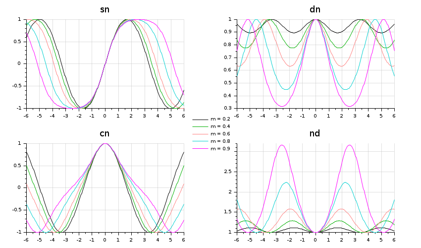
// Input data
x = linspace(-6,6,300)';
m = [0.2 0.4 0.6 0.8 0.9];
f = ["sn" "dn" "cn" "nd"];

// Computation
st = struct();
for i = 1:length(m)
    st(i) = ellipj(f,x,m(i));
end

// Plot
clf
for i = 1:size(f,"*")
    subplot(2,2,i)
    y = matrix(list2vec(st(f(i))), -1, length(m));
    plot2d(x, y,[1 14 28 18 6])
    title(f(i), "fontsize",4)
    xgrid(color("grey75"),1,7)
end

legend(gca(), msprintf("m =%4.1f\n",m'),1, %f);
lg = gce();
lg.legend_location = "by_coordinates";
lg.position = [-0.095 -0.08];
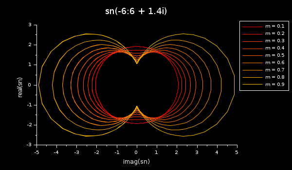
With some complex input numbers:
x = linspace(-6,6,300)';
m = 0.1:0.1:0.9;
sn = [];
for i = 1:length(m)
    sn(:,i) = ellipj(x+1.4*%i, m(i));
end

clf
plot2d(imag(sn), real(sn))
title("sn(-6:6 + 1.4i)", "fontsize",4)
xlabel("imag(sn)", "fontsize",2);
ylabel("real(sn)", "fontsize",2);
colordef(gcf(),"none")
gca().data_bounds(1:2) = [-5 5];
gca().tight_limits(1) = "on";
isoview
legend(gca(), msprintf("m =%4.1f\n",m'),"out_upper_right");
See also
- amell — ヤコビのam関数
- delip — 第一種の完全および不完全楕円積分
- %k — ヤコビの完全楕円積分
- Tee, Garry J.: Continuous branches of inverses of the 12 Jacobi elliptic functions for real argument”. 1997
History
| バージョン | 記述 |
| 6.1.0 | ellipj() introduced. |
| Report an issue | ||
| << dlgamma | Special Functions | erf >> |