Please note that the recommended version of Scilab is 2026.1.0. This page might be outdated.
See the recommended documentation of this function
csim
線形システムのシミュレーション (時間応答)
呼び出し手順
[y [,x]]=csim(u,t,sl,[x0 [,tol]])
引数
- u
関数, リストまたは文字列 (制御入力)
- t
時間を指定するための実数ベクトルで、
t(1)は 初期時間 (x0=x(t(1)))を表す.- sl
連続時間系の
syslinリスト (SIMO線形システム)- y
y=[y(t(i)], i=1,..,n となる行列- x
x=[x(t(i)], i=1,..,n となる行列- tol
2つの要素 [atol rtol] からなるベクトルであり、それぞれ ODEソルバ(ode参照)の絶対許容誤差および相対許容誤差を定義する
説明
線形制御系 slのシミュレーションを行います.
ただし,slは,
syslinリストで表された連続時間システムとします.
u は制御入力,x0 は状態量初期値です.
y は出力,x は状態量です.
制御入力は以下のいずれかとすることができます:
1. 関数 : [inputs]=u(t)
2. リスト : list(ut,parameter1,....,parametern).
ただし、inputs=ut(t,parameter1,....,parametern) (ut は関数)
3. インパルス応答の計算を表す文字列 "impuls"
(ここで,slの入力は単一でx0=0が必要).
直達項を有する系の場合, t=0における無限インパルスは無視されます.
4. ステップ応答の計算を表す文字列 "step"
(ここで、slの入力は単一で,x0=0が必要)
5. t の各値に対応する u の値を指定するベクトル.
例
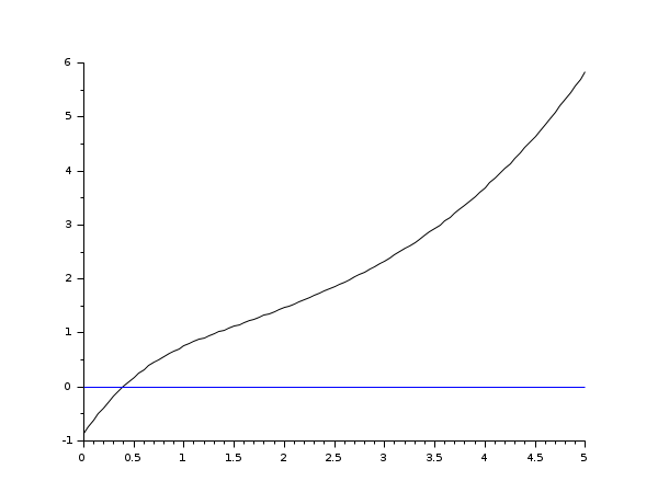
s=poly(0,'s');
rand('seed',0);
w=ssrand(1,1,3);
w('A')=w('A')-2*eye();
t=0:0.05:5;
//impulse(w) = step (s * w)
plot2d([t',t'],[(csim('step',t,tf2ss(s)*w))',0*t'])

s=poly(0,'s');
rand('seed',0);
w=ssrand(1,1,3);
w('A')=w('A')-2*eye();
t=0:0.05:5;
plot2d([t',t'],[(csim('impulse',t,w))',0*t'])
s=poly(0,'s');
rand('seed',0);
w=ssrand(1,1,3);
w('A')=w('A')-2*eye();
t=0:0.05:5;
//step(w) = impulse (s^-1 * w)
plot2d([t',t'],[(csim('step',t,w))',0*t'])
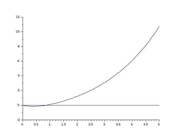
s=poly(0,'s');
rand('seed',0);
w=ssrand(1,1,3);
w('A')=w('A')-2*eye();
t=0:0.05:5;
plot2d([t',t'],[(csim('impulse',t,tf2ss(1/s)*w))',0*t'])

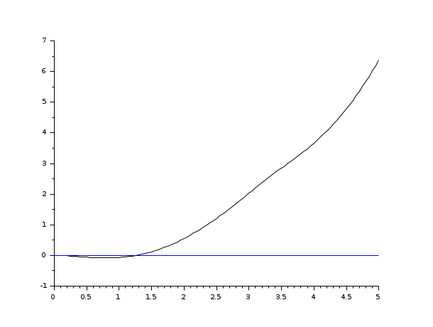
s=poly(0,'s');
rand('seed',0);
w=ssrand(1,1,3);
w('A')=w('A')-2*eye();
t=0:0.05:5;
//時間関数で定義された入力
deff('u=timefun(t)','u=abs(sin(t))')
clf();plot2d([t',t'],[(csim(timefun,t,w))',0*t'])
参照
| Report an issue | ||
| << arsimul | Time Domain | damp >> |