legendre

associated Legendre functions

Syntax

y = legendre(n, m, x)
y = legendre(n, m, x, normflag)

Arguments

n: non negative integer or vector of non negative integers regularly spaced with increment equal to 1
m: non negative integer or vector of non negative integers regularly spaced with increment equal to 1
x: real matrix(elements of x must be in the [-1,1] interval)
normflag: (optional) scalar string

Description

When n and m are scalars, legendre(n,m,x) evaluates the associated Legendre function Pnm(x) at all the elements of x. The definition used is :

$Pn|m(x)=(-1)^m.(1-x^2)^{m/2}.d^m[Pn(x)]/dx^m$

where Pn is the Legendre polynomial of degree n. So legendre(n,0,x) evaluates the Legendre polynomial Pn(x) at all the elements of x.

When the normflag is equal to "norm" you get a normalized version (without the (-1)^m factor), precisely :

$Pn|m(x,norm)=sqrt[(2n+1)/2 .(n-m)!/(n+m)!].(1-x^2)^{m/2}.d^m[Pn(x)]/dx^m$

which is useful to compute spherical harmonic functions (see Example 3):

For efficiency, one of the two first arguments may be a vector, for instance legendre(n1:n2,0,x) evaluates all the Legendre polynomials of degree n1, n1+1, ..., n2 at the elements of x and legendre(n,m1:m2,x) evaluates all the Legendre associated functions Pnm for m=m1, m1+1, ..., m2 at x.

Output format

In any case, the format of y is :

max(length(n),length(m)) x length(x)

and :

y(i,j) = P(n(i),m;x(j))   if n is a vector
y(i,j) = P(n,m(i);x(j))   if m is a vector
y(1,j) = P(n,m;x(j))      if both n and m are scalars

so that x is preferably a row vector but any mx x nx matrix is expected and considered as an 1 x (mx * nx) matrix, reshaped following the column order.

Examples

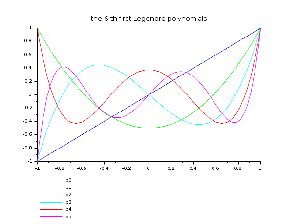
// example 1 : plot of the 6 first Legendre polynomials on (-1,1)
l = nearfloat("pred",1);
x = linspace(-l,l,200)';
y = legendre(0:5, 0,  x);
clf()
plot2d(x,y', leg="p0@p1@p2@p3@p4@p5@p6")
xtitle("the 6 th first Legendre polynomials")

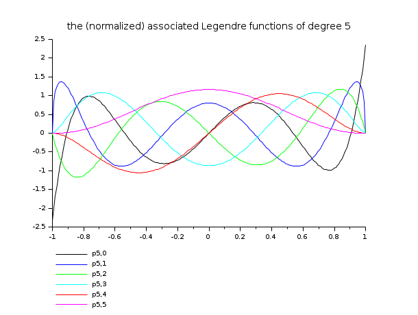
// example 2 : plot of the associated Legendre functions of degree 5
l = nearfloat("pred",1);
x = linspace(-l,l,200)';
y = legendre(5, 0:5, x, "norm");
clf()
plot2d(x,y', leg="p5,0@p5,1@p5,2@p5,3@p5,4@p5,5")
xtitle("the (normalized) associated Legendre functions of degree 5")

// example 3 : define then plot a spherical harmonic
// 3-1 : define the function Ylm
function [y]=Y(l, m, theta, phi)
  // theta may be a scalar or a row vector
  // phi may be a scalar or a column vector
  if m >= 0 then
     y = (-1)^m/(sqrt(2*%pi))*exp(%i*m*phi)*legendre(l, m, cos(theta), "norm")
  else
     y = 1/(sqrt(2*%pi))*exp(%i*m*phi)*legendre(l, -m, cos(theta), "norm")
  end
endfunction

// 3.2 : define another useful function
function [x, y, z]=sph2cart(theta, phi, r)
  // theta row vector      1 x nt
  // phi   column vector  np x 1
  // r     scalar or np x nt matrix (r(i,j) the length at phi(i) theta(j))
  x = r.*(cos(phi)*sin(theta));
  y = r.*(sin(phi)*sin(theta));
  z = r.*(ones(phi)*cos(theta));
endfunction

// 3-3 plot Y31(theta,phi)
l = 3; m = 1;
theta = linspace(0.1,%pi-0.1,60);
phi = linspace(0,2*%pi,120)';
f = Y(l,m,theta,phi);
[x1,y1,z1] = sph2cart(theta,phi,abs(f));       [xf1,yf1,zf1] = nf3d(x1,y1,z1);
[x2,y2,z2] = sph2cart(theta,phi,abs(real(f))); [xf2,yf2,zf2] = nf3d(x2,y2,z2);
[x3,y3,z3] = sph2cart(theta,phi,abs(imag(f))); [xf3,yf3,zf3] = nf3d(x3,y3,z3);

clf()
subplot(1,3,1)
plot3d(xf1,yf1,zf1,flag=[2 4 4]); xtitle("|Y31(theta,phi)|")
subplot(1,3,2)
plot3d(xf2,yf2,zf2,flag=[2 4 4]); xtitle("|Real(Y31(theta,phi))|")
subplot(1,3,3)
plot3d(xf3,yf3,zf3,flag=[2 4 4]); xtitle("|Imag(Y31(theta,phi))|")

Report an issue
<< gammaln	Fonctions spéciales	sinc >>

Copyright (c) 2022-2025 (Dassault Systèmes S.E.)
Copyright (c) 2017-2022 (ESI Group)
Copyright (c) 2011-2017 (Scilab Enterprises)
Copyright (c) 1989-2012 (INRIA)
Copyright (c) 1989-2007 (ENPC)
with contributors

Last updated:
Mon Jan 03 14:33:06 CET 2022