black

Arguments

sl

A siso or simo linear dynamical system, in state space, transfer function or zpk representations, in continuous or discrete time.

fmin,fmax

real scalars (frequency bounds)

frq

row vector or matrix (frequencies)

db, phi

row vectors or matrices of modulus (in dB) and phases (in degrees). One row for each response.

repf

row or matrix of complex frequency response(s). One row for each response.

step

real: (logarithmic) discretization step. See calfrq for the choice of default value.

comments

vector of character strings: captions.

Description

Black's diagram (Nichols'chart) for a linear dynamical system .

sl can be a continuous-time or discrete-time SIMO system given by its state space, rational transfer function (see syslin) or zpk representation. In case of multi-output the outputs are plotted with different colors.

The frequencies are given by the bounds fmin,fmax (in Hz) or by a row-vector (or a matrix for multi-output) frq.

To plot the grid of iso-gain and iso-phase of y/(1+y) use nicolschart().

Default values for fmin and fmax are 1.d-3, 1.d+3 if sl is continuous-time or 1.d-3, 0.5/sl.dt (nyquist frequency) if sl is discrete-time.

Examples

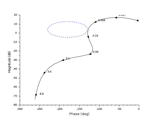
//Black diagram
s=poly(0,'s');
sl=syslin('c',5*(1+s)/(.1*s.^4+s.^3+15*s.^2+3*s+1))
clf();black(sl,0.01,10);

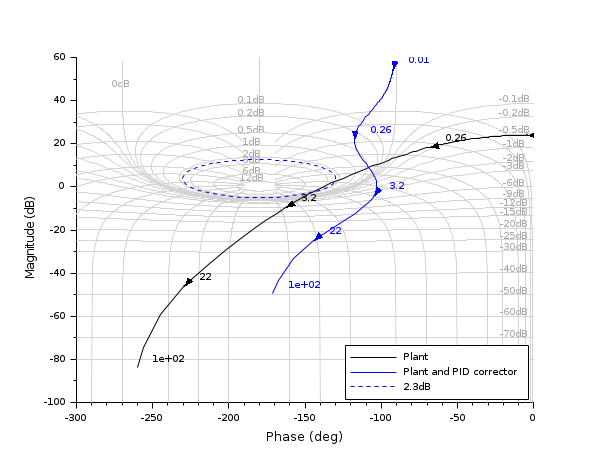
//Black diagram with Nichols chart as a grid
s=poly(0,'s');
Plant=syslin('c',16000/((s+1)*(s+10)*(s+100)));
//two degree of freedom PID
tau=0.2;xsi=1.2;
PID=syslin('c',(1/(2*xsi*tau*s))*(1+2*xsi*tau*s+tau.^2*s.^2));
clf();
black([Plant;Plant*PID ],0.01,100,["Plant";"Plant and PID corrector"]);
//move the caption in the lower right corner
ax=gca();Leg=ax.children(1);
Leg.legend_location="in_lower_right";
nicholschart(colors=color('light gray')*[1 1])

See also

• nicholschart — Nichols chart
• bode — Bode plot
• nyquist — nyquist plot
• syslin — linear system definition
• calfrq — frequency response discretization
• datatips — Tool for placing and editing tips along the plotted curves

History