Scilab 6.1.0
Please note that the recommended version of Scilab is 2026.1.0. This page might be outdated.
See the recommended documentation of this function
bode_asymp
ボード線図の漸近線
呼び出し手順
bode_asymp(sl)
bode_asymp(sl, wmin, wmax)
引数
- sl
syslinリスト (連続時間系のSISOまたはSIMO線形システム) (状態空間または有理型).- wmin, wmax
実スカラー: 周波数領域の下限および上限 (単位: rad/s).
説明
システムslの漸近線をプロットします.
オプション引数 wmin および wmax (単位:rad/s)
により漸近線をプロットする際に周波数範囲を指定することができます.
 |
 | 警告: 最初の入力引数が実数行列の場合,この関数は適用できません. |
例
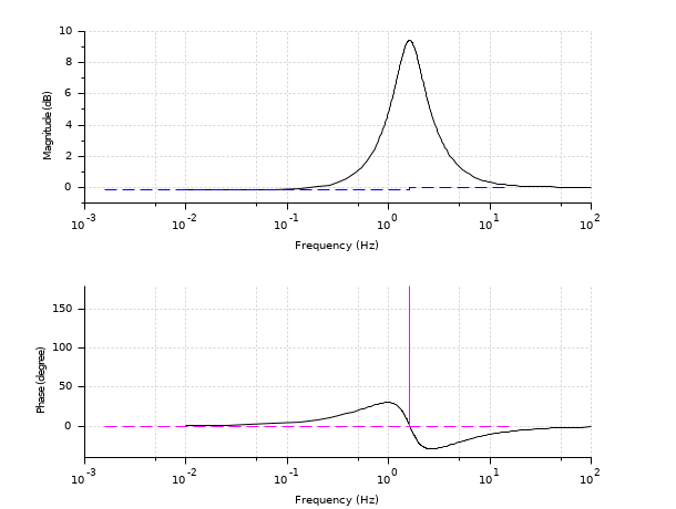
s = poly(0, "s");
h = syslin("c", (s^2+2*0.9*10*s+100)/(s^2+2*0.3*10.1*s+102.01));
clf(); bode(h, 0.01, 100); bode_asymp(h);
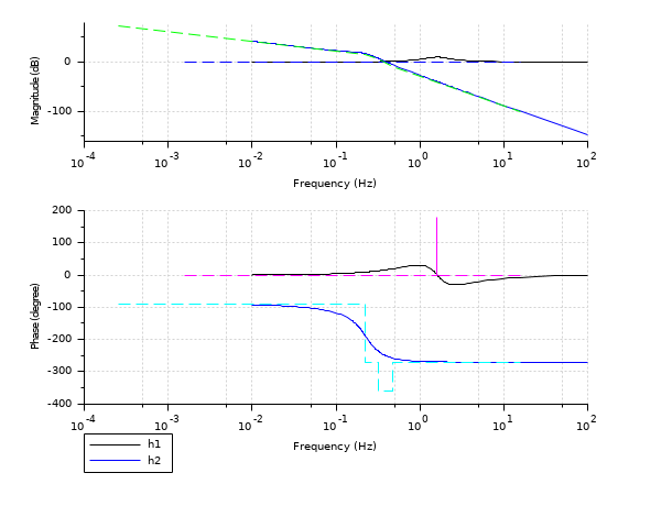
s = poly(0, "s");
h1 = syslin("c", (s^2+2*0.9*10*s+100)/(s^2+2*0.3*10.1*s+102.01));
h2 = syslin("c", (10*(s+3))/(s*(s+2)*(s^2+s+2)));
clf(); bode([h1; h2], 0.01, 100, ["h1"; "h2"]); bode_asymp([h1; h2]);
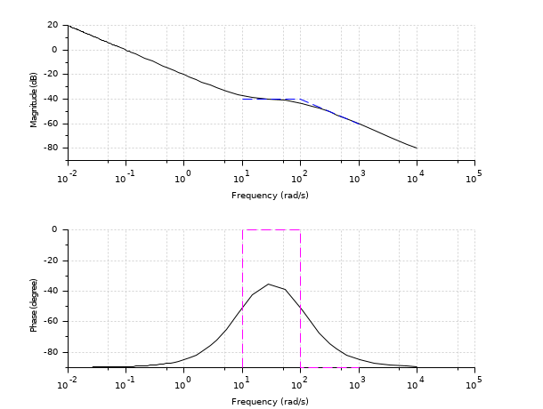
s = %s;
G = (s+10)/(s*(s+100)); // 有理行列
sys = syslin("c", G); // 伝達関数表現の連続時間線形系
f_min = .0001; f_max = 1600; // 単位: Hz
clf(); bode(sys, f_min, f_max, "rad"); // オプション引数 "rad" は Hzをrad/sに変換します
bode_asymp(sys, 10, 1000); // 指定した範囲(単位:rad/s)で漸近線をプロット
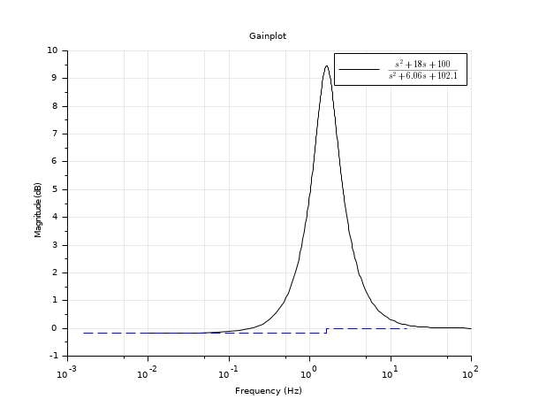
s = poly(0, "s");
h = syslin("c", (s^2+2*0.9*10*s+100)/(s^2+2*0.3*10.1*s+102.01));
h = tf2ss(h);
clf();
gainplot(h, 0.01, 100, "$\frac{s^2+18 s+100}{s^2+6.06 s+102.1}$"); // 単位: ヘルツ
bode_asymp(h)
参照
履歴
| Version | Description |
| 5.5.0 | bode_asymp() 関数が導入されました. |
| Report an issue | ||
| << bode | Frequency Domain | calfrq >> |