Scilab 6.0.2
- Scilabヘルプ
- Graphics
- 2d_plot
- champ
- champ1
- champ_properties
- comet
- contour2d
- contour2di
- contour2dm
- contourf
- errbar
- fchamp
- fec
- fec_properties
- fgrayplot
- fplot2d
- grayplot
- grayplot_properties
- graypolarplot
- histplot
- LineSpec
- Matplot
- Matplot1
- Matplot_properties
- paramfplot2d
- plot
- plot2d
- plot2d2
- plot2d3
- plot2d4
- polarplot
- scatter
- Sfgrayplot
- Sgrayplot
Please note that the recommended version of Scilab is 2026.1.0. This page might be outdated.
See the recommended documentation of this function
plot2d3
2次元プロット (垂直棒グラフ)
呼び出し手順
plot2d3([logflags,] x,y,[style,strf,leg,rect,nax])
plot232(y)
plot2d3(x,y <,opt_args>)
引数
- args
パラメータの説明については
plot2d参照.
説明
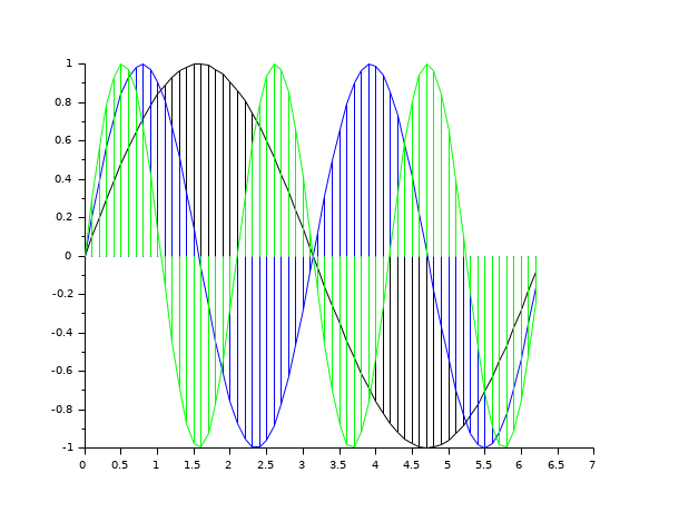
plot2d3 はplot2d と同じですが,
曲線が垂直棒グラフとしてプロットされます.
デフォルトで, 連続するプロットは重ね描きされます.前のプロットを消去するには
clf()を使用してください.
コマンド plot2d3() を入力するとデモを参照できます.
 | plot2dxx (xx = 1 から 4)により提供されるモードは全て
plot2dを用いて,
polyline_styleオプションを対応する数字に設定することにより,
有効にすることができます. |
例
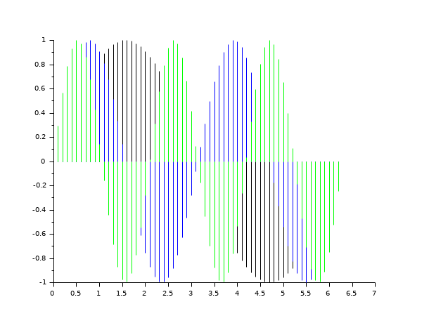
clf()
x = [0:0.1:2*%pi]';
plot2d(x, [sin(x) sin(2*x) sin(3*x)])
e = gce();
e.children(1).polyline_style=3;
e.children(2).polyline_style=3;
e.children(3).polyline_style=3;
参照
- plot2d — 2Dプロット
- plot2d2 — 2次元プロット (階段状関数)
- plot2d4 — 2次元プロット (矢印形式)
- clf — Clears and resets a figure or a frame uicontrol
- polyline_properties — Polylineエンティティプロパティの説明
| Report an issue | ||
| << plot2d2 | 2d_plot | plot2d4 >> |