- Aide de Scilab
- Fonctions Elémentaires
- Nombres complexes
- Mathématiques discrètes
- Matrices élémentaires
- Exponentielle
- Virgule flottante
- Bases de numération
- Manipulation de matrices
- Opérations matricielles
- Chercher et trier
- Opérations sur les ensembles
- Traitement du signal
- Calcul symbolique
- Trigonométrie
- Bitwise operations
- and
- &
- lstsize
- modulo
- or
- |
- sign
- size
- cat
- cell2mat
- cellstr
- iscolumn
- isempty
- isequal
- ismatrix
- isrow
- isscalar
- issquare
- isvector
- ndims
- nthroot
- num2cell
- unwrap
Please note that the recommended version of Scilab is 2026.1.0. This page might be outdated.
See the recommended documentation of this function
unwrap
unwrap a Y(x) profile or a Z(x,y) surface. Unfold a Y(x) profile
Calling Sequences
unwrap() // runs some examples
[U, breakPoints] = unwrap(Y)
[U, breakPoints] = unwrap(Y, z_jump)
[U, cuspPoints]  = unwrap(Y, "unfold")
U = unwrap(Z)
U = unwrap(Z, z_jump)
U = unwrap(Z, z_jump, dir)
Arguments
- Y
Vector of real numbers: the profile to unwrap or unfold. Implicit abscissae X are assumed to be equispaced.
- Z
Matrix of real numbers: the surface to unwrap. Implicit abscissae (X,Y) are assumed to be cartesian and equispaced (constant steps may be different along X versus along Y).
- z_jump
Scalar real positive number used in unwrapping mode: the jump's height applied at breakpoints, performing the unwrapping. Only its absolute value is considered. The jump actually applied has the sign of the slope on both sides of each breakpoint. The default value is
z_jump = 2*%pi. The special valuez_jump = 0applies jumps equal to the average slope around each breakpoint, restoring a continuous slope over the whole profile or surface.- dir
"c" | "r" | "" (default): direction along which unwrapping is performed. "c" unwraps along columns, "r" unwraps along rows, "" unwraps in both directions.
- "unfold"
Provide this switch to unfold the given curve if it is folded, instead of unwrapping it.
- U
Unwrapped profile or surface, or unfolded profile.
Uhas the same sizes asYorZ.- breakPoints, cuspPoints
Vector of indices of points in
Ywhere wrapping or folding has been detected and processed.
Description
UNWRAPPING
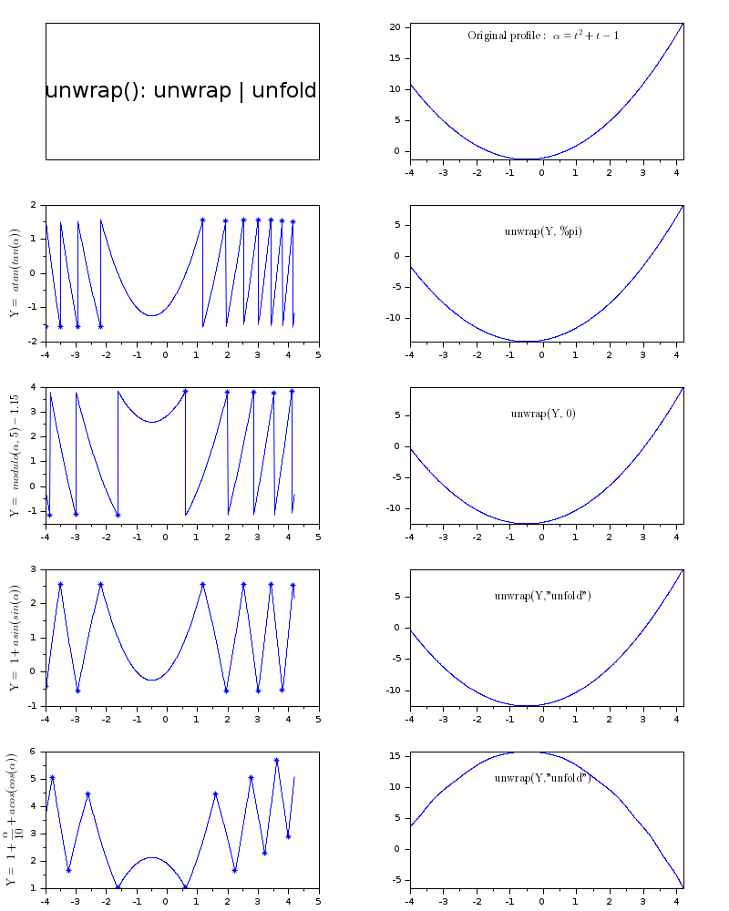
unwrap() will be useful to process profiles or even surfaces wrapped for instance by a periodic and monotonic function such as
Y = modulo(X,w) or Y = atan(tan(X)). It aims to somewhat invert these functions, recovering the input X over it full range instead of the limited w or [-%pi/2, %pi/2] one.
A breakpoint of a wrapped profile is detected as a point where slopes on both neighbouring sides of the point are almost equal but much smaller (in absolute value) from and opposite to the slope at the considered point: at the point, there is a jump breaking and opposed to the neighbouring slope.
This detection strategy avoids considering any particular level as a wrapping one. It allows to process wrapped profiles to which a constant (or even a trend) has been added afterwards.
Unwrapping consists in reducing every detected jump and somewhat restoring a continuous slope (initially assumed to be so). At each point, it is performed by applying a Y-shift on a whole side of the profile, with respect to the other. The Y-shift may be the same for all breakpoints, as provided by the user. If the user specifies a null Y-shift, unwrap() applies a jump equal to the average neighbouring slope, depending on each breakpoint.
 | An unwrapped profile is always defined but for a constant. |
Unless dir is used, unwrap() applied to a surface unwraps its first column. Each point of this one is then taken as reference level for unwrapping each line starting with it.
UNFOLDING
If the "unfold" keyword is used and a profile -- not a surface -- is provided, the profile is assumed to be folded instead of being wrapped.
At a folding point -- or "cusp point" --, the profile is continuous, but its slope is broken: the slope has almost the same absolute value on both sides of the point, but is somewhat opposed from one side to the other.
Folding may occur for instance when a non-monotonic periodic function and its inverse are applied to a profile X, like with Y= acos(cos(X)). Recovering X from Y is quite more difficult than if it was wrapped. Indeed, some ambiguous situations may exist, like when the profile is tangentially folded on one of its quasi-horizontal sections (if any).
When a cusp point is detected, a) one side of the profile starting from it is opposed (upside down), and b) the continuity of the profile and of its slope are preserved and retrieved at the considered point (this may need adding a small jump by the local slope).
| The slope on the left edge of the input profile is used as starting reference. The unfolded profile may be upside down with respect to the original true one. In addition, as for unwrapping, it is defined but for a constant. |
Known limitations: presently, folded surfaces can't be processed.
Examples
Unwrapping or unfolding 1D profiles:
// 1D EXAMPLES
// -----------
f = scf();
f.figure_size = [800 1000];
f.figure_position(2) = 0;
f.figure_name = "unwrap() & ""unfold""" + _(": 1-D examples ");
ax = gda();
ax.y_label.font_size=2;
drawlater()

// Original 1D profile
t = linspace(-4,4.2,800);
alpha = t.^2 + t -1;
subplot(5,2,1)
titlepage("unwrap(): unwrap | unfold")
subplot(5,2,2)
plot(t,alpha)
t2 = "$\text{Original profile: } \alpha=t^2+t-1$";
ax = gca();
ax.tight_limits = "on";
yT = max(alpha) - strange(alpha)*0.1;
xstring(0,yT,t2)
e = gce();
e.text_box_mode = "centered";
e.font_size = 2;

// Loop over cases
for i=1:4
    subplot(5,2,2*i+1)
    if i==1 then
        // Wrapping by atan(tan())
        ralpha = atan(tan(alpha));            // Raw recovered alpha [pi]
        ylabel("$atan(tan(\alpha))$")
        [u, K] = unwrap(ralpha, %pi);         // arctan
        t2 = "$\text{unwrap(Y, \%pi)}$";
    elseif i==2
        // Wrapping by modulo() + Y-shift
        c = (rand(1,1)-0.5)*4;
        ralpha = pmodulo(alpha, 5) + c;
        ylabel("$modulo(\alpha,\ 5)"+msprintf("%+5.2f",c)+"$")
        [u, K] = unwrap(ralpha, 0);
        t2 = "$\text{unwrap(Y, 0)}$";
    elseif i==3
        // Folding by asin(sin()) + Y-shift
        ralpha = 1+asin(sin(alpha));          // Raw recovered alpha [2.pi]
        ylabel("$1+asin(sin(\alpha))$")
        [u, K] = unwrap(ralpha, "unfold");
        t2 = "$\text{unwrap(Y,""unfold"")}$";
    else
        // Folding by acos(cos()) + a trend
        ralpha = 1+alpha/10+acos(cos(alpha)); // Raw recovered alpha [2.pi]
        ylabel("$1+\frac{\alpha}{10}+acos(cos(\alpha))$")
        [u, K] = unwrap(ralpha, "unfold");
        t2 = "$\text{unwrap(Y,""unfold"")}$";
    end
    // Plotting the profile to be processed
    plot(t, ralpha)
    // Staring the breakpoints or the cusp points on the curve:
    if K~=[] then
        plot(t(K), ralpha(K),"*")
    end
    // Plotting the processed (unwrapped/unfolded) profile:
    subplot(5,2,2*i+2)
    plot(t,u)
    ax = gca();
    ax.tight_limits = "on";
    // Adding a legend:
    yT = max(u) - strange(u)*0.2;
    xstring(0,yT,t2)
    e = gce();
    e.text_box_mode = "centered";
    e.font_size = 2;
end
sda();
drawnow()
Unwrapping 2-D surfaces:
// 2-D EXAMPLES
// -----------
ax = gda();
ax.title.font_size = 2;
f = scf();
f.color_map = hotcolormap(100);
f.figure_size = [475 1050];
f.figure_position(2) = 0;
f.figure_name = "unwrap()" + _(": 2-D examples");
drawlater()

nx = 300;
ny = 400;
rmax = 8.8;
x = linspace(-rmax/2, rmax/2, nx)-1;
y = linspace(-rmax/2, rmax/2, ny)+1;
[X, Y] = meshgrid(x,y);
for ex=0:1   // examples
    // Original surface
        // Generating the surface
    if ex==0 then
        z = X.^2 + Y.^2;
    else
        z = sqrt(0.3+sinc(sqrt(z)*3))*17-7;
    end
    // PLotting it in 3D
    subplot(4,2,1+ex)
    surf(x, y, z)
    title("Original profile Z")
    e = gce();
    e.thickness = 0; // removes the mesh
    e.parent.tight_limits = "on";

    // Wrapped surface (flat)
    m = 2.8;
    zw = pmodulo(z, m); // wraps it
    subplot(4,2,3+ex)
    grayplot(x, y, zw')
    title(msprintf("Zw = pmodulo(Z, %g)  (flat)",m))
    ax0 = gca();
    ax0.tight_limits = "on";

    // Unwrapped surfaces (flat):
    // in both directions:
    u = unwrap(zw, 0);
    subplot(4,2,5+ex)
    grayplot(x, y, u')
    title(msprintf("unwrap(Zw, %g)  (flat)", 0))
    ax3 = gca();
    ax3.tight_limits = "on";

    if ex==0 then
        direc = "r";
    else
        direc = "c";
    end
    // Along a single direction:
    u = unwrap(zw, m, direc);
    subplot(4,2,7+ex)
    grayplot(x, y, u')
    title(msprintf("unwrap(Zw, %g, ""%s"")  (flat)",m,direc))
    ax1 = gca();
    ax1.tight_limits = "on";
end
sda();
drawnow()
See Also
History
| Version | Description |
| 5.5.0 | unwrap() function introduced |
| Report an issue | ||
| << num2cell | Fonctions Elémentaires | Algèbre Lineaire >> |