Please note that the recommended version of Scilab is 2026.1.0. This page might be outdated.
See the recommended documentation of this function
fminsearch
Computes the unconstrained minimimum of given function with the Nelder-Mead algorithm.
SYNOPSIS
x = fminsearch ( costf , x0 )
x = fminsearch ( costf , x0 , options )
[x,fval] = fminsearch ( costf , x0 , options )
[x,fval,exitflag] = fminsearch ( costf , x0 , options )
[x,fval,exitflag,output] = fminsearch ( costf , x0 , options )
Description
This function searches for the unconstrained minimum of a given cost function.
The provided algorithm is a direct search algorithm, i.e. an algorithm which does not use the derivative of the cost function. It is based on the update of a simplex, which is a set of k>=n+1 vertices, where each vertex is associated with one point and one function value. This algorithm is the Nelder-Mead algorithm.
See the demonstrations, in the Optimization section, for an overview of this component.
See the "Nelder-Mead User's Manual" on Scilab's wiki and on the Scilab forge for further information.
Design
This function is based on a specialized use of the more general neldermead component. Users which want to have a more flexible solution based on direct search algorithms should consider using the neldermead component instead of the fminsearch function.
Arguments
- costf
a function or a list, the objective function. This function computes the value of the cost function.
See below for the details of the communication between the optimization system and the cost function.
- x0
a matrix of doubles, the initial guess.
- options
A struct which contains configurable options of the algorithm (see below for details).
- x
The minimum.
- fval
The minimum function value.
- exitflag
The flag associated with exist status of the algorithm.
The following values are available.
- -1
The maximum number of iterations has been reached.
- 0
The maximum number of function evaluations has been reached.
- 1
The tolerance on the simplex size and function value delta has been reached. This signifies that the algorithm has converged, probably to a solution of the problem.
- output
A struct which stores detailed information about the exit of the algorithm. This struct contains the following fields.
- output.algorithm
A string containing the definition of the algorithm used, i.e. 'Nelder-Mead simplex direct search'.
- output.funcCount
The number of function evaluations.
- output.iterations
The number of iterations.
- output.message
A string containing a termination message.
The cost function
The costf argument to configure the cost function. The cost
function is used to compute the objective function value f.
The cost function must have the following header :
f = costf ( x )
where
- x
the current point
- f
the value of the cost function
It might happen that the function requires additional arguments to be evaluated.
In this case, we can use the following feature.
The argument costf can also be the list (myfun,a1,a2,...).
In this case myfun, the first element in the list, must be a function and must
have the header:
f = myfun ( x, a1, a2, ...)
a1, a2, ...
are automatically appended at the end of the calling sequence.Options
In this section, we describe the options input argument which have an effect on the algorithm used by fminsearch.
The options input argument is a data structure which drives the behaviour of fminsearch. It allows to handle several options in a consistent and simple interface, without the problem of managing many input arguments.
These options must be set with the optimset function. See the optimset help for details of the options managed by this function.
The fminsearch function is sensitive to the following options.
- options.MaxIter
The maximum number of iterations. The default is 200 * n, where n is the number of variables.
- options.MaxFunEvals
The maximum number of evaluations of the cost function. The default is 200 * n, where n is the number of variables.
- options.TolFun
The absolute tolerance on function value. The default value is 1.e-4.
- options.TolX
The absolute tolerance on simplex size. The default value is 1.e-4.
- options.Display
The verbose level. Possible values are "notify", "iter", "final" and "off". The default value is "notify".
- options.OutputFcn
The output function, or a list of output functions. The default value is empty.
- options.PlotFcns
The plot function, or a list of plotput functions. The default value is empty.
Termination criteria
In this section, we describe the termination criteria used by fminsearch.
The criteria is based on the following variables:
- ssize
the current simplex size,
- shiftfv
the absolute value of the difference of function value between the highest and lowest vertices.
If both the following conditions
ssize < options.TolX
and
shiftfv < options.TolFun
are true, then the iterations stop.
The size of the simplex is computed using the "sigmaplus" method of the optimsimplex component. The "sigmamplus" size is the maximum length of the vector from each vertex to the first vertex. It requires one loop over the vertices of the simplex.
The initial simplex
The fminsearch algorithm uses a special initial simplex, which is an heuristic depending on the initial guess. The strategy chosen by fminsearch corresponds to the -simplex0method flag of the neldermead component, with the "pfeffer" method. It is associated with the -simplex0deltausual = 0.05 and -simplex0deltazero = 0.0075 parameters. Pfeffer's method is a heuristic which is presented in "Global Optimization Of Lennard-Jones Atomic Clusters" by Ellen Fan. It is due to L. Pfeffer at Stanford. See in the help of optimsimplex for more details.
The number of iterations
In this section, we present the default values for the number of iterations in fminsearch.
The options input argument is an optional data structure which can contain the options.MaxIter field. It stores the maximum number of iterations. The default value is 200n, where n is the number of variables. The factor 200 has not been chosen by chance, but is the result of experiments performed against quadratic functions with increasing space dimension.
This result is presented in "Effect of dimensionality on the nelder-mead simplex method" by Lixing Han and Michael Neumann. This paper is based on Lixing Han's PhD, "Algorithms in Unconstrained Optimization". The study is based on numerical experiment with a quadratic function where the number of terms depends on the dimension of the space (i.e. the number of variables). Their study shows that the number of iterations required to reach the tolerance criteria is roughly 100n. Most iterations are based on inside contractions. Since each step of the Nelder-Mead algorithm only require one or two function evaluations, the number of required function evaluations in this experiment is also roughly 100n.
Output and plot functions
The optimset function can be used to configure one or more output and plot functions.
The output function is expected to have the following header:
stop = myoutputfun ( x , optimValues , state )
The input arguments x, optimValues
and state are described in detail in the optimset
help page.
Set the stop boolean variable to false to continue the optimization and
set it to true to interrupt the optimization.
The optimValues.procedure field represent the type of step
used during the current iteration and can be equal to one
of the following strings
"" (the empty string),
"initial simplex",
"expand",
"reflect",
"contract inside",
"contract outside".
The plot function is expected to have the following header:
myplotfun ( x , optimValues , state )
where the input arguments x, optimValues
and state have the same definition as for the output function.
Example
In the following example, we use the fminsearch function to compute the minimum of the Rosenbrock function. We first define the function "banana", and then use the fminsearch function to search the minimum, starting with the initial guess [-1.2 1.0]. In this particular case, 85 iterations are performed and 159 function evaluations are
function y=banana(x)
  y = 100*(x(2)-x(1)^2)^2 + (1-x(1))^2;
endfunction
[x, fval, exitflag, output] = fminsearch ( banana , [-1.2 1] )
Example with customized options
In the following example, we configure the absolute tolerance
on the size of the simplex to a larger value, so that the algorithm
performs less iterations. Since the default value of "TolX" for the
fminsearch function is 1.e-4, we decide to use 1.e-2.
The optimset function is used to create an
optimization data structure and the field associated with the string "TolX"
is set to 1.e-2. The opt data structure is then
passed to the fminsearch function as the third
input argument.
In this particular case, the number of iterations is 70
with 130 function evaluations.
function y=banana(x)
  y = 100*(x(2)-x(1)^2)^2 + (1-x(1))^2;
endfunction
opt = optimset ( "TolX" , 1.e-2 );
[x , fval , exitflag , output] = fminsearch ( banana , [-1.2 1] , opt )
Example with a pre-defined plot function
In the following example, we want to produce a graphic of the
progression of the algorithm, so that we can include that graphic
into a report without defining a customized plot function.
The fminsearch function comes with the
following 3 pre-defined functions :
optimplotfval, which plots the function value,
optimplotx, which plots the current point
x,optimplotfunccount, which plots the number of function evaluations.
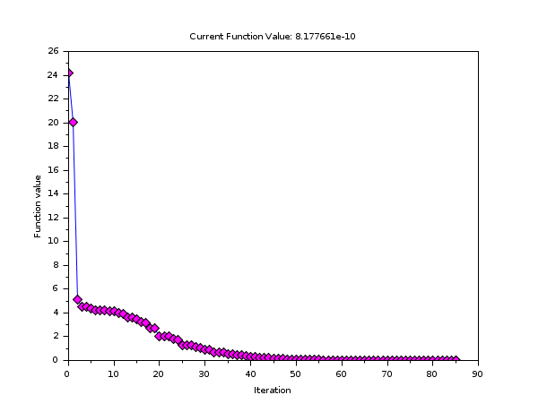
In the following example, we use the three pre-defined functions in order to create one graphic, representing the function value depending on the number of iterations.
function y=banana(x)
  y = 100*(x(2)-x(1)^2)^2 + (1-x(1))^2;
endfunction
opt = optimset ( "PlotFcns" , optimplotfval );
[x fval] = fminsearch ( banana , [-1.2 1] , opt );
In the previous example, we could replace the "optimplotfval" function with "optimplotx" or "optimplotfunccount" and obtain different results. In fact, we can get all the figures at the same time, by setting the "PlotFcns" to a list of functions, as in the following example.
function y=banana(x)
  y = 100*(x(2)-x(1)^2)^2 + (1-x(1))^2;
endfunction
myfunctions = list ( optimplotfval , optimplotx , optimplotfunccount );
opt = optimset ( "PlotFcns" , myfunctions );
[x fval] = fminsearch ( banana , [-1.2 1] , opt );
Example with a customized output function
In the following example, we want to produce intermediate
outputs of the algorithm. We define the outfun
function, which takes the current point x as input argument.
The function plots the current point into the current graphic window
with the plot function.
We use the "OutputFcn" feature of the optimset function
and set it to the output function. Then the option data structure is passed to the
fminsearch function. At each iteration, the output
function is called back, which creates and update an interactive plot.
While this example creates a 2D plot, the user may customized the
output function so that it writes a message in the console, write some
data into a data file, etc... The user can distinguish
between the output function (associated with the "OutputFcn" option)
and the plot function (associated with the "PlotFcns" option).
See the optimset for more details on this feature.
Example with customized "Display"
The "Display" option allows to get some input about the intermediate steps of the algorithm as well as to be warned in case of a convergence problem.
In the following example, we present what happens in case of a convergence problem. We set the number of iterations to 10, instead of the default 400 iterations. We know that 85 iterations are required to reach the convergence criteria. Therefore, the convergence criteria is not met and the maximum number of iterations is reached.
function y=banana(x)
  y = 100*(x(2)-x(1)^2)^2 + (1-x(1))^2;
endfunction
opt = optimset ( "MaxIter" , 10 );
[x fval] = fminsearch ( banana , [-1.2 1] , opt );
Since the default value of the "Display" option is "notify", a message is generated, which warns the user about a possible convergence problem. The previous script produces the following output.
Exiting: Maximum number of iterations has been exceeded
- increase MaxIter option.
Current function : 4.1355598
Notice that if the "Display" option is now set to "off", no message is displayed at all. Therefore, the user should be warned that turning the Display "off" should be used at your own risk...
In the following example, we present how to display intermediate steps used by the algorithm. We simply set the "Display" option to the "iter" value.
function y=banana(x)
  y = 100*(x(2)-x(1)^2)^2 + (1-x(1))^2;
endfunction
opt = optimset ( "Display" , "iter" );
[x fval] = fminsearch ( banana , [-1.2 1] , opt );
The previous script produces the following output. It allows to see the number of function evaluations, the minimum function value and which type of simplex step is used for the iteration.
Iteration   Func-count     min f(x)         Procedure
0            3             24.2
1            3            20.05         initial simplex
2            5         5.161796         expand
3            7         4.497796         reflect
4            9         4.497796         contract outside
5           11        4.3813601         contract inside
etc...
Example with customized output
In this section, we present an example where all the fields from the optimValues
data structure are used to print a message at each iteration.
function stop=outfun(x, optimValues, state)
  fc = optimValues.funccount;
  fv = optimValues.fval;
  it = optimValues.iteration;
  pr = optimValues.procedure;
  mprintf ( "%d %e %d -%s-\n" , fc , fv , it , pr )
  stop = %f
endfunction
opt = optimset ( "OutputFcn" , outfun );
[x fval] = fminsearch ( banana , [-1.2 1] , opt );
The previous script produces the following output.
3 2.420000e+001 0 --
3 2.005000e+001 1 -initial simplex-
5 5.161796e+000 2 -expand-
7 4.497796e+000 3 -reflect-
9 4.497796e+000 4 -contract outside-
11 4.381360e+000 5 -contract inside-
13 4.245273e+000 6 -contract inside-
[...]
157 1.107549e-009 84 -contract outside-
159 8.177661e-010 85 -contract inside-
159 8.177661e-010 85 --
Passing extra parameters
In the following example, we solve a modified Rosenbrock test case.
Notice that the objective function has two extra parameters
a and b.
This is why the costf argument is set as a list,
where the first element is the function and the
remaining elements are the extra parameters.
function y=bananaext(x, a, b)
  y = a*(x(2)-x(1)^2)^2 + (b-x(1))^2;
endfunction
a = 100;
b = 12;
xopt = [12  144]
fopt = 0
[x fval] = fminsearch ( list(bananaext,a,b) , [10 100] )
Some advices
In this section, we present some practical advices with respect to the Nelder-Mead method. A deeper analysis is provided in the bibliography at the end of this help page, as well as in the "Nelder-Mead User's Manual" provided on Scilab's Wiki. The following is a quick list of tips to overcome problems that may happen with this algorithm.
We should consider the optim function before considering the
fminsearchfunction. Because optim uses the gradient of the function and uses this information to guess the local curvature of the cost function, the number of iterations and function evaluations is (much) lower with optim, when the function is sufficiently smooth. If the derivatives of the function are not available, it is still possible to use numerical derivatives combined with the optim function: this feature is provided by the numderivative function. If the function has discontinuous derivatives, the optim function provides thendsolver which is very efficient. Still, there are situations where the cost function is discontinuous or "noisy". In these situations, thefminsearchfunction can perform well.We should not expected a fast convergence with many parameters, i.e. more that 10 to 20 parameters. It is known that the efficiency of this algorithm decreases rapidly when the number of parameters increases.
The default tolerances are set to pretty loose values. We should not reduce the tolerances in the goal of getting very accurate results. Because the convergence rate of Nelder-Mead's algorithm is low (at most linear), getting a very accurate solution will require a large number of iterations. Instead, we can most of the time expect a "good reduction" of the cost function with this algorithm.
Although the algorithm practically converges in many situations, the Nelder-Mead algorithm is not a provably convergent algorithm. There are several known counter-examples where the algorithm fails to converge on a stationnary point and, instead, converge to a non-stationnary point. This situation is often indicated by a repeated application of the contraction step. In that situation, we simply restart the algorithm with the final point as the new initial guess. If the algorithm converges to the same point, there is a good chance that this point is a "good" solution.
Taking into account for bounds constraints or non-linear inequality constraints can be done by penalization methods, i.e. setting the function value to a high value when the constraints are not satisfied. While this approach works in some situations, it may also fail. In this case, users might be interested in Box's complex algorithm, provided by Scilab in the
neldermeadcomponent. If the problem is really serious, Box's complex algorithm will also fail and a more powerful solver is necessary.
Bibliography
"Sequential Application of Simplex Designs in Optimisation and Evolutionary Operation", Spendley, W. and Hext, G. R. and Himsworth, F. R., American Statistical Association and American Society for Quality, 1962
"A Simplex Method for Function Minimization", Nelder, J. A. and Mead, R., The Computer Journal, 1965
"Iterative Methods for Optimization", C. T. Kelley, SIAM Frontiers in Applied Mathematics, 1999
"Algorithm AS47 - Function minimization using a simplex procedure", O'Neill, R., Applied Statistics, 1971
"Effect of dimensionality on the nelder-mead simplex method", Lixing Han and Michael Neumann, Optimization Methods and Software, 21, 1, 1--16, 2006.
"Algorithms in Unconstrained Optimization", Lixing Han, Ph.D., The University of Connecticut, 2000.
"Global Optimization Of Lennard-Jones Atomic Clusters" Ellen Fan, Thesis, February 26, 2002, McMaster University
"Nelder Mead's User Manual", Consortium Scilab - Digiteo, Michael Baudin, 2010
See Also
- optim — non-linear optimization routine
- neldermead — Provides direct search optimization algorithms.
- optimset — Configures and returns an optimization data structure.
- optimget — Queries an optimization data structure.
- optimplotfval — Plot the function value of an optimization algorithm
- optimplotx — Plot the value of the parameters of an optimization algorithm
- optimplotfunccount — Plot the number of function evaluations of an optimization algorithm
| Report an issue | ||
| << Neldermead | Neldermead | neldermead >> |