Please note that the recommended version of Scilab is 2026.1.0. This page might be outdated.
See the recommended documentation of this function
optim
non-linear optimization routine
Calling Sequence
fopt = optim(costf, x0)
fopt = optim(costf [,<contr>],x0 [,algo] [,df0 [,mem]] [,work] [,<stop>] [,<params>] [,imp=iflag])
[fopt, xopt] = optim(...)
[fopt, xopt, gopt] = optim(...)
[fopt, xopt, gopt, work] = optim(...)
[fopt, xopt, gopt, work, iters] = optim(...)
[fopt, xopt, gopt, work, iters, evals] = optim(...)
[fopt, xopt, gopt, work, iters, evals, err] = optim(...)
[fopt, xopt, [gopt, work, iters, evals, err], ti, td] = optim(..., params="si","sd")
Arguments
- costf
a function, a list or a string, the objective function.
- x0
real vector, the initial guess for
x.- <contr>
an optional sequence of arguments containing the lower and upper bounds on
x. If bounds are required, this sequence of arguments must be"b",binf,bsupwherebinfandbsupare real vectors with same dimension asx0.- algo
a string, the algorithm to use (default
algo="qn").The available algorithms are:
"qn": Quasi-Newton with BFGS"gc": limited memory BFGS"nd": non-differentiable.The
"nd"algorithm does not accept bounds onx.The
"qn"cannot be used ifsize(x0)>46333.
- df0
real scalar, a guess of the decreasing of
fat first iteration. (defaultdf0=1).- mem
integer, the number of variables used to approximate the Hessian (default
mem=10). This feature is available for the"gc"algorithm without constraints and the non-smooth algorithm"nd"without constraints.- <stop>
a sequence of arguments containing the parameters controlling the convergence of the algorithm. The following sequences are available:
"ar",nap
"ar",nap,iter
"ar",nap,iter,epsg
"ar",nap,iter,epsg,epsf
"ar",nap,iter,epsg,epsf,epsx
where:
- nap
maximum number of calls to
costfallowed (defaultnap=100).- iter
maximum number of iterations allowed (default
iter=100).- epsg
threshold on gradient norm (default
epsg= %eps).- epsf
threshold controlling decreasing of
f(defaultepsf=0).- epsx
threshold controlling variation of
x(defaultepsx=0). This vector (possibly matrix) with same size asx0can be used to scalex.
- <params>
in the case where the objective function is a C or Fortran routine, a sequence of arguments containing the method to communicate with the objective function. This option has no meaning when the cost function is a Scilab script.
The available values for <params> are the following.
"in"That mode allows to allocate memory in the internal Scilab workspace so that the objective function can get arrays with the required size, but without directly allocating the memory. The
"in"value stands for "initialization". In that mode, before the value and derivative of the objective function is to be computed, there is a dialog between theoptimScilab primitive and the objective functioncostf. In this dialog, the objective function is called two times, with particular values of theindparameter. The first time,indis set to 10 and the objective function is expected to set thenizs,nrzsandndzsinteger parameters of thenirdcommon, which is defined as:common /nird/ nizs,nrzs,ndzs
This allows Scilab to allocate memory inside its internal workspace. The second time the objective function is called,
indis set to 11 and the objective function is expected to set theti,trandtzarrays. After this initialization phase, each time it is called, the objective function is ensured that theti,trandtzarrays which are passed to it have the values that have been previously initialized."ti",valtiIn this mode,
valtiis expected to be a Scilab vector variable containing integers. Whenever the objective function is called, thetiarray it receives contains the values of the Scilab variable."td", valtdIn this mode,
valtdis expected to be a Scilab vector variable containing double values. Whenever the objective function is called, thetdarray it receives contains the values of the Scilab variable."ti",valti,"td",valtdThis mode combines the two previous modes.
"si"In this mode,
valtiis saved in the output variableti."sd"In this mode,
valtdis saved in the output variabletd."si","sd"This mode combines the two previous modes.
The
ti, tdarrays may be used so that the objective function can be computed. For example, if the objective function is a polynomial, the ti array may may be used to store the coefficients of that polynomial.Users should choose carefully between the
"in"mode and the"ti"and"td"mode, depending on the fact that the arrays are Scilab variables or not. If the data is available as Scilab variables, then the"ti", valti, "td", valtdmode should be chosen. If the data is available directly from the objective function, the"in"mode should be chosen. Notice that there is no"tr"mode, since, in Scilab, all real values are doubles.If neither the "in" mode, nor the "ti", "td" mode is chosen, that is, if <params> is not present as an option of the optim primitive, the user may should not assume that the ti,tr and td arrays can be used : reading or writing the arrays may generate unpredictable results.
- "imp=iflag"
named argument used to set the trace mode (default
imp=0, which prints no messages). Ifimpis greater or equal to 1, more information are printed, depending on the algorithm chosen. More precisely:"qn"without constraints: fromiflag=1toiflag=3.iflag>=1: initial and final print,iflag>=2: one line per iteration (number of iterations, number of calls to f, value of f),iflag>=3: extra information on line searches.
"qn"with bounds constraints: fromiflag=1toiflag=4.iflag>=1: initial and final print,iflag>=2: one line per iteration (number of iterations, number of calls to f, value of f),iflag>=3: extra information on line searches.
"gc"without constraints: fromiflag=1toiflag=5.iflag>=1andiflag>=2: initial and final print,iflag=3: one line per iteration (number of iterations, number of calls to f, value of f),iflag>=4: extra information on lines searches.
"gc"with bounds constraints: fromiflag=1toiflag=3.iflag>=1: initial and final print,iflag>=2: one print per iteration,iflag=3: extra information.
"nd"with bounds constraints: fromiflag=1toiflag=8.iflag>=1: initial and final print,iflag>=2: one print on each convergence,iflag>=3: one print per iteration,iflag>=4: line search,iflag>=5: various tolerances,iflag>=6: weight and information on the computation of direction.
If
impis lower than 0, then the cost function is evaluated every-miterations, withind=1.- fopt
the value of the objective function at the point
xopt- xopt
best value of
xfound.- gopt
the gradient of the objective function at the point
xopt- work
working array for hot restart for quasi-Newton method. This array is automatically initialized by
optimwhenoptimis invoked. It can be used as input parameter to speed-up the calculations.- iters
scalar, the number of iterations that is displayed when
imp=2.- evals
scalar, the number of
costfunction evaluations that is displayed whenimp=2.- err
scalar, a termination indicator. The success flag is
9.err=1: Norm of projected gradient lower than...err=2: At last iteration f decreases by less than...err=3: Optimization stops because of too small variations for x.err=4: Optim stops: maximum number of calls to f is reached.err=5: Optim stops: maximum number of iterations is reached.err=6: Optim stops: too small variations in gradient direction.err=7: Stop during calculation of descent direction.err=8: Stop during calculation of estimated hessian.err=9: End of optimization, successful completion.err=10: End of optimization (linear search fails).
Description
This function solves unconstrained nonlinear optimization problems:
min f(x)
where x is a vector and f(x)
is a function that returns a scalar. This function can also solve bound
constrained nonlinear optimization problems:
min f(x)
binf <= x <= bsup
where binf is the lower bound and
bsup is the upper bound on x.
The costf argument can be a Scilab function, a
list or a string giving the name of a C or Fortran routine (see
"external"). This external must return the value f of
the cost function at the point x and the gradient
g of the cost function at the point
x.
- Scilab function case
If
costfis a Scilab function, its calling sequence must be:[f, g, ind] = costf(x, ind)
where
xis the current point,indis an integer flag described below,fis the real value of the objective function at the pointxandgis a vector containing the gradient of the objective function atx. The variableindis described below.- List case
It may happen that objective function requires extra arguments. In this case, we can use the following feature. The
costfargument can be the list(real_costf, arg1,...,argn). In this case,real_costf, the first element in the list, must be a Scilab function with calling sequence:The[f,g,ind]=real_costf(x,ind,arg1,...,argn)x,f,g,indarguments have the same meaning as before. In this case, each time the objective function is called back, the argumentsarg1,...,argnare automatically appended at the end of the calling sequence ofreal_costf.- String case
If
costfis a string, it refers to the name of a C or Fortran routine which must be linked to Scilab- Fortran case
The calling sequence of the Fortran subroutine computing the objective must be:
subroutine costf(ind,n,x,f,g,ti,tr,td)
with the following declarations:
integer ind,n ti(*)
double precision x(n),f,g(n),td(*)
real tr(*)
The argument
indis described below.If ind = 2, 3 or 4, the inputs of the routine are :
x, ind, n, ti, tr,td.If ind = 2, 3 or 4, the outputs of the routine are :
fandg.- C case
The calling sequence of the C function computing the objective must be:
void costf(int *ind, int *n, double *x, double *f, double *g, int *ti, float *tr, double *td)
The argument
indis described below.The inputs and outputs of the function are the same as in the fortran case.
On output, ind<0 means that
f cannot be evaluated at x and
ind=0 interrupts the optimization.
Termination criteria
Each algorithm has its own termination criteria, which may use the
parameters given by the user, that is nap,
iter, epsg, epsf
and epsx. Not all the parameters are taken into
account. In the table below, we present the specific termination
parameters which are taken into account by each algorithm. The
unconstrained solver is identified by "UNC" while the bound constrained
solver is identified by "BND". An empty entry means that the parameter is
ignored by the algorithm.
| Solver | nap | iter | epsg | epsf | epsx |
| optim/"qn" UNC | X | X | X | ||
| optim/"qn" BND | X | X | X | X | X |
| optim/"gc" UNC | X | X | X | X | |
| optim/"gc" BND | X | X | X | X | X |
| optim/"nd" UNC | X | X | X | X |
Example: Scilab function
The following is an example with a Scilab function. Notice, for simplifications reasons, the Scilab function "cost" of the following example computes the objective function f and its derivative no matter of the value of ind. This allows to keep the example simple. In practical situations though, the computation of "f" and "g" may raise performances issues so that a direct optimization may be to use the value of "ind" to compute "f" and "g" only when needed.
function [f, g, ind]=cost(x, ind)
    xref = [1; 2; 3];
    f = 0.5 * norm(x - xref)^2;
    g = x - xref;
endfunction

// Simplest call
x0 = [1; -1; 1];
[fopt, xopt] = optim(cost, x0)

// Use "gc" algorithm
[fopt, xopt, gopt] = optim(cost, x0, "gc")

// Use "nd" algorithm
[fopt, xopt, gopt] = optim(cost, x0, "nd")

// Upper and lower bounds on x
[fopt, xopt, gopt] = optim(cost, "b", [-1;0;2], [0.5;1;4], x0)

// Upper and lower bounds on x and setting up the algorithm to "gc"
[fopt, xopt, gopt] = optim(cost, "b", [-1; 0; 2], [0.5; 1; 4], x0, "gc")

// Bound on the number of calls to the objective function
[fopt, xopt, gopt] = optim(cost, "b", [-1; 0; 2], [0.5; 1; 4], x0, "gc", "ar", 3)

// Set max number of calls to the objective function (3)
// Set max number of iterations (100)
// Set stopping threshold on the value of f (1e-6),
// on the value of the norm of the gradient of the objective function (1e-6)
// on the improvement on the parameters x_opt (1e-6;1e-6;1e-6)
[fopt, xopt, gopt] = optim(cost, "b", [-1; 0; 2], [0.5; 1; 4], x0, "gc", "ar", 3, 100, 1e-6, 1e-6, [1e-3; 1e-3; 1e-3])

// Additional messages are printed in the console.
[fopt, xopt] = optim(cost, x0, imp = 3)
Example: Print messages
The imp flag may take negative integer values,
say k. In that case, the cost function is called once every -k iterations.
This allows to draw the function value or write a log file.
This feature is available only with the "qn"
algorithm without constraints.
In the following example, we solve the Rosenbrock test case. For each iteration of the algorithm, we print the value of x, f and g.
function [f, g, ind]=cost(x, ind)
    xref = [1; 2; 3];
    f = 0.5 * norm(x - xref)^2;
    g = x - xref;
    if (ind == 1) then
        mprintf("f(x) = %s, |g(x)|=%s\n", string(f), string(norm(g)))
    end
endfunction

x0 = [1; -1; 1];
[fopt, xopt] = optim(cost, x0, imp = -1)
The previous script produces the following output.
-->[fopt, xopt] = optim(cost, x0, imp = -1)
f(x) = 6.5, |g(x)|=3.6055513
f(x) = 2.8888889, |g(x)|=2.4037009
f(x) = 9.861D-31, |g(x)|=1.404D-15
f(x) = 0, |g(x)|=0
Norm of projected gradient lower than   0.0000000D+00.

 xopt  =

    1.
    2.
    3.
 fopt  =

    0.
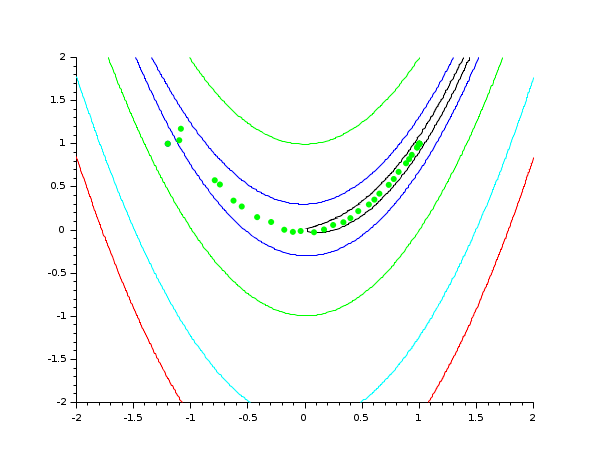
In the following example, we solve the Rosenbrock test case. For each iteration of the algorithm, we plot the current value of x into a 2D graph containing the contours of Rosenbrock's function. This allows to see the progress of the algorithm while the algorithm is performing. We could as well write the value of x, f and g into a log file if needed.
// 1. Define Rosenbrock for optimization
function [f, g, ind]=rosenbrock(x, ind)
    f = 100.0 *(x(2) - x(1)^2)^2 + (1 - x(1))^2;
    g(1) = - 400. * (x(2) - x(1)**2) * x(1) -2. * (1. - x(1))
    g(2) = 200. * (x(2) - x(1)**2)
endfunction

// 2. Define rosenbrock for contouring
function f=rosenbrockC(x1, x2)
    x = [x1 x2]
    ind = 4
    [f, g, ind] = rosenbrock (x, ind)
endfunction

// 3. Define Rosenbrock for plotting
function [f, g, ind]=rosenbrockPlot(x, ind)
    [f, g, ind] = rosenbrock (x, ind)
    if (ind == 1) then
        plot (x(1), x(2), "g.")
    end
endfunction

// 4. Draw the contour of Rosenbrock's function
x0 = [-1.2 1.0];
xopt = [1.0 1.0];
xdata = linspace(-2,2,100);
ydata = linspace(-2,2,100);
contour (xdata, ydata, rosenbrockC, [1 10 100 500 1000])
plot(x0(1), x0(2), "b.")
plot(xopt(1), xopt(2), "r*")

// 5. Plot the optimization process, during optimization
[fopt, xopt] = optim (rosenbrockPlot, x0, imp = -1)
Example: Optimizing with numerical derivatives
It is possible to optimize a problem without an explicit knowledge
of the derivative of the cost function. For this purpose, we can use the
numderivative function to compute a numerical derivative of the
cost function.
In the following example, we use the numderivative function to solve
Rosenbrock's problem.
function f=rosenbrock(x)
    f = 100.0 *(x(2)-x(1)^2)^2 + (1-x(1))^2;
endfunction

function [f, g, ind]=rosenbrockCost(x, ind)
    f = rosenbrock (x);
    g = numderivative (rosenbrock, x);
endfunction

x0 = [-1.2 1.0];

[fopt, xopt] = optim (rosenbrockCost, x0)
Example: Counting function evaluations and number of iterations
The imp option can take negative values. If the
imp is equal to m where
m is a negative integer, then the cost function is
evaluated every -m iterations, with the
ind input argument equal to 1. The following example
uses this feature to compute the number of iterations. The global variable
mydata is used to store the number of function
evaluations as well as the number of iterations.
function [f, g, ind]=cost(x, ind)
    global _MYDATA_
    if (ind == 1)
        _MYDATA_.niter = _MYDATA_.niter + 1;
    end
    _MYDATA_.nfevals = _MYDATA_.nfevals + 1;
    xref = [1; 2; 3];
    if (ind == 2 | ind == 4) then
        f = 0.5*norm(x-xref)^2;
    else
        f = 0;
    end
    if (ind == 3 | ind == 4) then
        g = x-xref;
    else
        g = zeros(3, 1);
    end
endfunction

x0 = [1; -1; 1];
global _MYDATA_
_MYDATA_ = tlist (["MYDATA", "niter", "nfevals"]);
_MYDATA_.niter = 0;
_MYDATA_.nfevals = 0;

[f, xopt] = optim(cost, x0, imp=-1);
mprintf ("Number of function evaluations: %d\n", _MYDATA_.nfevals);
mprintf ("Number of iterations: %d\n", _MYDATA_.niter);
While the previous example perfectly works, there is a risk that the
same variable _MYDATA_ is used by some internal
function used by optim. In this case, the value may be
wrong. This is why a sufficiently weird variable name has been
used.
Example : Passing extra parameters
In most practical situations, the cost function depends on extra parameters which are required to evaluate the cost function. There are several methods to achieve this goal.
In the following example, the cost function uses 4 parameters
a, b, c and d. We define the cost
function with additional input arguments, which are declared after the
index argument. Then we pass a list as the first input argument of the
optim solver. The first element of the list is the cost
function. The additional variables are directly passed to the cost
function.
function [f, g, ind]=costfunction(x, ind, a, b, c, d)
    f = a * (x(1) - c) ^2 + b * (x(2) - d)^2
    g(1) = 2 * a * (x(1) - c)
    g(2) = 2 * b * (x(2) - d)
endfunction

x0 = [1 1];
a = 1.0;
b = 2.0;
c = 3.0;
d = 4.0;
costf = list (costfunction, a, b, c, d);
[fopt, xopt] = optim (costf, x0, imp = 2)
In complex cases, the cost function may have so many parameters, that having a function which takes all arguments as inputs is not convenient. For example, consider the situation where the cost function needs 12 parameters. Then, designing a function with 14 input arguments (x, index and the 12 parameters) is difficult to manage. Instead, we can use a more complex data structure to store our data. In the following example, we use a tlist to store the 4 input arguments. This method can easily be expanded to an arbitrary number of parameters.
function [f, g, ind]=costfunction(x, ind, parameters)
    // Get the parameters
    a = parameters.a
    b = parameters.b
    c = parameters.c
    d = parameters.d
    f = a * (x(1) - c) ^2 + b * (x(2) - d)^2
    g(1) = 2 * a * (x(1) - c)
    g(2) = 2 * b * (x(2) - d)
endfunction

x0 = [1 1];
a = 1.0;
b = 2.0;
c = 3.0;
d = 4.0;
// Store the parameters
parameters = tlist ([
"T_MYPARAMS"
"a"
"b"
"c"
"d"
]);

parameters.a = a;
parameters.b = b;
parameters.c = c;
parameters.d = d;
costf = list (costfunction, parameters);
[fopt, xopt] = optim (costf, x0, imp = 2)
In the following example, the parameters are defined before the optimizer is called. They are directly used in the cost function.
// The example NOT to follow
function [f, g, ind]=costfunction(x, ind)
    f = a * (x(1) - c) ^2 + b * (x(2) - d)^2
    g(1) = 2 * a * (x(1) - c)
    g(2) = 2 * b * (x(2) - d)
endfunction
x0 = [1 1];
a = 1.0;
b = 2.0;
c = 3.0;
d = 4.0;
[fopt, xopt] = optim (costfunction, x0, imp = 2)
While the previous example perfectly works, there is a risk that the
same variables are used by some internal function used by
optim. In this case, the value of the parameters are
not what is expected and the optimization can fail or, worse, give a wrong
result. It is also difficult to manage such a function, which requires
that all the parameters are defined in the calling context.
In the following example, we define the cost function with the
classical header. Inside the function definition, we declare that the
parameters a, b, c and d are global
variables. Then we declare and set the global variables.
// Another example NOT to follow
function [f, g, ind]=costfunction(x, ind)
    global a b c d
    f = a * (x(1) - c) ^2 + b * (x(2) - d)^2
    g(1) = 2 * a * (x(1) - c)
    g(2) = 2 * b * (x(2) - d)
endfunction
x0 = [1 1];
global a b c d
a = 1.0;
b = 2.0;
c = 3.0;
d = 4.0;
[fopt, xopt] = optim (costfunction, x0, imp = 2)
While the previous example perfectly works, there is a risk that the
same variables are used by some internal function used by
optim. In this case, the value of the parameters are
not what is expected and the optimization can fail or, worse, give a wrong
result.
Example : Checking that derivatives are correct
Many optimization problem can be avoided if the derivatives are computed correctly. One common reason for failure in the step-length procedure is an error in the calculation of the cost function and its gradient. Incorrect calculation of derivatives is by far the most common user error.
In the following example, we give a false implementation of
Rosenbrock's gradient. In order to check the computation of the
derivatives, we use the numderivative function. We define
the simplified function, which delegates the
computation of f to the rosenbrock function. The
simplified function is passed as an input argument of
the numderivative function.
function [f, g, index]=rosenbrock(x, index)
    f = 100.0 *(x(2)-x(1)^2)^2 + (1-x(1))^2;
    // Exact :
    g(1) = - 400. * (x(2) - x(1)**2) * x(1) -2. * (1. - x(1))
    // Wrong :
    g(1) = - 1200. * (x(2) - x(1)**2) * x(1) -2. * (1. - x(1))
    g(2) = 200. * (x(2) - x(1)**2)
endfunction

function f=simplified(x)
    index = 1;
    [f, g, index] = rosenbrock (x, index)
endfunction

x0 = [-1.2 1];
index = 1;
[f, g, index] = rosenbrock (x0, index);
gnd = numderivative (simplified, x0.');
mprintf("Exact derivative:[%s]\n", strcat (string(g), " "));
mprintf("Numerical derivative:[%s]\n", strcat (string(gnd), " "));
The previous script produces the following output. Obviously, the difference between the two gradient is enormous, which shows that the wrong formula has been used in the gradient.
Exact derivative:[-638 -88]
Numerical derivative:[-215.6 -88]
Example: C function
The following is an example with a C function, where a C source code is written into a file, dynamically compiled and loaded into Scilab, and then used by the "optim" solver. The interface of the "rosenc" function is fixed, even if the arguments are not really used in the cost function. This is because the underlying optimization solvers must assume that the objective function has a known, constant interface. In the following example, the arrays ti and tr are not used, only the array "td" is used, as a parameter of the Rosenbrock function. Notice that the content of the arrays ti and td are the same that the content of the Scilab variable, as expected.
// External function written in C (C compiler required)
// write down the C code (Rosenbrock problem)
C=['#include <math.h>'
'double sq(double x)'
'{ return x*x;}'
'void rosenc(int *ind, int *n, double *x, double *f, double *g, '
'                                int *ti, float *tr, double *td)'
'{'
'  double p;'
'  int i;'
'  p=td[0];'
'  if (*ind==2||*ind==4) {'
'    *f=1.0;'
'    for (i=1;i<*n;i++)'
'      *f+=p*sq(x[i]-sq(x[i-1]))+sq(1.0-x[i]);'
'  }'
'  if (*ind==3||*ind==4) {'
'    g[0]=-4.0*p*(x[1]-sq(x[0]))*x[0];'
'    for (i=1;i<*n-1;i++)'
'      g[i]=2.0*p*(x[i]-sq(x[i-1]))-4.0*p*(x[i+1]-sq(x[i]))*x[i]-2.0*(1.0-x[i]);'
'    g[*n-1]=2.0*p*(x[*n-1]-sq(x[*n-2]))-2.0*(1.0-x[*n-1]);'
'  }'
'}'];
cd TMPDIR;
mputl(C, TMPDIR+'/rosenc.c')

// compile the C code
l = ilib_for_link('rosenc', 'rosenc.c', [], 'c');

// incremental linking
link(l, 'rosenc', 'c')

//solve the problem
x0 = [40; 10; 50];
p = 100;
[f, xo, go] = optim('rosenc', x0, 'td', p)
Example: Fortran function
The following is an example with a Fortran function.
// External function written in Fortran (Fortran compiler required)
// write down the Fortran  code (Rosenbrock problem)
F = ['      subroutine rosenf(ind, n, x, f, g, ti, tr, td)'
'      integer ind,n,ti(*)'
'      double precision x(n),f,g(n),td(*)'
'      real tr(*)'
'c'
'      double precision y,p'
'      p=td(1)'
'      if (ind.eq.2.or.ind.eq.4) then'
'        f=1.0d0'
'        do i=2,n'
'          f=f+p*(x(i)-x(i-1)**2)**2+(1.0d0-x(i))**2'
'        enddo'
'      endif'
'      if (ind.eq.3.or.ind.eq.4) then'
'        g(1)=-4.0d0*p*(x(2)-x(1)**2)*x(1)'
'        if(n.gt.2) then'
'          do i=2,n-1'
'            g(i)=2.0d0*p*(x(i)-x(i-1)**2)-4.0d0*p*(x(i+1)-x(i)**2)*x(i)'
'     &           -2.0d0*(1.0d0-x(i))'
'          enddo'
'        endif'
'        g(n)=2.0d0*p*(x(n)-x(n-1)**2)-2.0d0*(1.0d0-x(n))'
'      endif'
'      return'
'      end'];
cd TMPDIR;
mputl(F, TMPDIR+'/rosenf.f')

// compile the Fortran code
l = ilib_for_link('rosenf', 'rosenf.f', [], 'f');

// incremental linking
link(l, 'rosenf', 'f')

//solve the problem
x0 = [40; 10; 50];
p = 100;
[f, xo, go] = optim('rosenf', x0, 'td', p)
Example: Fortran function with initialization
The following is an example with a Fortran function in which the "in" option is used to allocate memory inside the Scilab environment. In this mode, there is a dialog between Scilab and the objective function. The goal of this dialog is to initialize the parameters of the objective function. Each part of this dialog is based on a specific value of the "ind" parameter.
At the beginning, Scilab calls the objective function, with the ind parameter equal to 10. This tells the objective function to initialize the sizes of the arrays it needs by setting the nizs, nrzs and ndzs integer parameters of the "nird" common. Then the objective function returns. At this point, Scilab creates internal variables and allocate memory for the variable izs, rzs and dzs. Scilab calls the objective function back again, this time with ind equal to 11. This tells the objective function to initialize the arrays izs, rzs and dzs. When the objective function has done so, it returns. Then Scilab enters in the real optimization mode and calls the optimization solver the user requested. Whenever the objective function is called, the izs, rzs and dzs arrays have the values that have been previously initialized.
//
// Define a fortran source code and compile it (fortran compiler required)
//
fortransource = ['      subroutine rosenf(ind,n,x,f,g,izs,rzs,dzs)'
'C     -------------------------------------------'
'c     Example of cost function given by a subroutine'
'c     if n<=2 returns ind=0'
'c     f.bonnans, oct 86'
'      implicit double precision (a-h,o-z)'
'      real rzs(1)'
'      double precision dzs(*)'
'      dimension x(n),g(n),izs(*)'
'      common/nird/nizs,nrzs,ndzs'
'      if (n.lt.3) then'
'        ind=0'
'        return'
'      endif'
'      if(ind.eq.10) then'
'         nizs=2'
'         nrzs=1'
'         ndzs=1'
'         return'
'      endif'
'      if(ind.eq.11) then'
'         izs(1)=5'
'         izs(2)=10'
'         dzs(1)=100.0d+0'
'         return'
'      endif'
'      if(ind.eq.2)go to 5'
'      if(ind.eq.3)go to 20'
'      if(ind.eq.4)go to 5'
'      ind=-1'
'      return'
'5     f=1.0d+0'
'      do 10 i=2,n'
'        im1=i-1'
'10      f=f + dzs(1)*(x(i)-x(im1)**2)**2 + (1.0d+0-x(i))**2'
'      if(ind.eq.2)return'
'20    g(1)=-4.0d+0*dzs(1)*(x(2)-x(1)**2)*x(1)'
'      nm1=n-1'
'      do 30 i=2,nm1'
'        im1=i-1'
'        ip1=i+1'
'        g(i)=2.0d+0*dzs(1)*(x(i)-x(im1)**2)'
'30      g(i)=g(i) -4.0d+0*dzs(1)*(x(ip1)-x(i)**2)*x(i) - '
'     &        2.0d+0*(1.0d+0-x(i))'
'      g(n)=2.0d+0*dzs(1)*(x(n)-x(nm1)**2) - 2.0d+0*(1.0d+0-x(n))'
'      return'
'      end'];
cd TMPDIR;
mputl(fortransource, TMPDIR + '/rosenf.f')

// compile the C code
libpath = ilib_for_link('rosenf', 'rosenf.f', [], 'f');

// incremental linking
linkid = link(libpath, 'rosenf', 'f');

x0 = 1.2 * ones(1, 5);
//
// Solve the problem
//
[f, x, g] = optim('rosenf', x0, 'in');
Example: Fortran function with initialization on Windows with Intel Fortran Compiler
Under the Windows operating system with Intel Fortran Compiler, one must carefully design the fortran source code so that the dynamic link works properly. On Scilab's side, the optimization component is dynamically linked and the symbol "nird" is exported out of the optimization dll. On the cost function's side, which is also dynamically linked, the "nird" common must be imported in the cost function dll.
The following example is a re-writing of the previous example, with special attention for the Windows operating system with Intel Fortran compiler as example. In that case, we introduce additional compiling instructions, which allows the compiler to import the "nird" symbol.
fortransource = ['subroutine rosenf(ind,n,x,f,g,izs,rzs,dzs)'
'cDEC$ IF DEFINED (FORDLL)'
'cDEC$ ATTRIBUTES DLLIMPORT:: /nird/'
'cDEC$ ENDIF'
'C     -------------------------------------------'
'c     Example of cost function given by a subroutine'
'c     if n<=2 returns ind=0'
'c     f.bonnans, oct 86'
'      implicit double precision (a-h,o-z)'
[etc...]
Example: Fortran function with tab saving
Adding the "si" and/or "sd" options to optim implies
the addition of the output arguments "ti" and/or "td", which will represent
the working tables of the objective function.
Those output arguments must be placed at the end of the output list.
// Move into the temporary directory to create the temporary files there
cur_dir = pwd();
chdir(TMPDIR);
fortransource = ['      subroutine rosenf(ind,n,x,f,g,izs,rzs,dzs)'
'C     -------------------------------------------'
'c (DLL Digital Visual Fortran)'
'c On Windows, we need to import common nird from scilab'
'cDEC$ IF DEFINED (FORDLL)'
'cDEC$ ATTRIBUTES DLLIMPORT:: /nird/'
'cDEC$ ENDIF'
'C     -------------------------------------------'
'c     Example of cost function given by a subroutine'
'c     if n.le.2 returns ind=0'
'c     f.bonnans, oct 86'
'      implicit double precision (a-h,o-z)'
'      real rzs(1)'
'      double precision dzs(*)'
'      dimension x(n),g(n),izs(*)'
'      common/nird/nizs,nrzs,ndzs'
'      if (n.lt.3) then'
'        ind=0'
'        return'
'      endif'
'      if(ind.eq.10) then'
'         nizs=2'
'         nrzs=1'
'         ndzs=1'
'         return'
'      endif'
'      if(ind.eq.11) then'
'         izs(1)=5'
'         izs(2)=10'
'         dzs(1)=100.0d+0'
'         return'
'      endif'
'      if(ind.eq.2)go to 5'
'      if(ind.eq.3)go to 20'
'      if(ind.eq.4)go to 5'
'      ind=-1'
'      return'
'5     f=1.0d+0'
'      do 10 i=2,n'
'        im1=i-1'
'10      f=f + dzs(1)*(x(i)-x(im1)**2)**2 + (1.0d+0-x(i))**2'
'      if(ind.eq.2)return'
'20    g(1)=-4.0d+0*dzs(1)*(x(2)-x(1)**2)*x(1)'
'      nm1=n-1'
'      do 30 i=2,nm1'
'        im1=i-1'
'        ip1=i+1'
'        g(i)=2.0d+0*dzs(1)*(x(i)-x(im1)**2)'
'30      g(i)=g(i) -4.0d+0*dzs(1)*(x(ip1)-x(i)**2)*x(i) - '
'     &        2.0d+0*(1.0d+0-x(i))'
'      g(n)=2.0d+0*dzs(1)*(x(n)-x(nm1)**2) - 2.0d+0*(1.0d+0-x(n))'
'      return'
'      end'];
mputl(fortransource, TMPDIR + '/rosenf.f');
ilib_for_link('rosenf', 'rosenf.f', [], 'f');
exec loader.sce;
chdir(cur_dir);
//
// Define some constants
//
Leps = 10e3 * 8.e-5;
bs = 10.*ones(1, 5);
bi = -bs;
x0 = 0.12 * bs;
epsx = 1.e-15 * x0;
xopt = .1*bs;

// 'ti' and 'td' always at the end of the output sequence
[f, x, ti, td]                           = optim('rosenf', x0, 'in', 'si', 'sd')
[f, x, g, ti, td]                        = optim('rosenf', x0, 'in', 'si', 'sd')
[f, x, g, w, ti, td]                     = optim('rosenf', x0, 'in', 'si', 'sd')
[f, x, g, w, niter, nevals, ti, td]      = optim('rosenf', x0, 'in', 'si', 'sd')
[f, x, g, w, niter, nevals, err, ti, td] = optim('rosenf', x0, 'in', 'si', 'sd')

// With input argument 'in', ti and td will be initialized by rosenf function.
[f, x, ti, td] = optim('rosenf', x0, 'in', 'si', 'sd')
// Reuses the last ti and td for the next call and return it again.
[f, x, ti, td] = optim('rosenf', x0, 'ti', ti, 'td', td, 'si', 'sd')

// Initializes ti and td but return only ti
[f, x, ti] = optim('rosenf', x0, 'in', 'si')
[f, x, ti] = optim('rosenf', x0, 'ti', ti, 'si')

// Initializes ti and td but return only td
[f, x, td] = optim('rosenf', x0, 'in', 'sd')
[f, x, td] = optim('rosenf', x0, 'td', td, 'sd')
See Also
- external — Scilab Object, external function or routine
- qpsolve — linear quadratic programming solver
- datafit — Parameter identification based on measured data
- leastsq — Solves non-linear least squares problems
- numderivative — approximate derivatives of a function (Jacobian or Hessian)
- NDcost — generic external for optim computing gradient using finite differences
References
The following is a map from the various options to the underlying solvers.
- "qn" without constraints
n1qn1 : a quasi-Newton method with a Wolfe-type line search
- "qn" with bounds constraints
qnbd : a quasi-Newton method with projection
RR-0242 - A variant of a projected variable metric method for bound constrained optimization problems, Bonnans Frederic, Rapport de recherche de l'INRIA - Rocquencourt, Octobre 1983
- "gc" without constraints
n1qn3 : a Quasi-Newton limited memory method with BFGS.
- "gc" with bounds constraints
gcbd : a BFGS-type method with limited memory and projection
- "nd" without constraints
n1fc1 : a bundle method
- "nd" with bounds constraints
not available
| Report an issue | ||
| << numderivative | Optimization and Simulation | qld >> |