Sgrayplot
smooth 2D plot of a surface using colors
Syntax
Sgrayplot(x, y, z, <opt_args>)
Sgrayplot(x, y, z [,strf, rect, nax, zminmax, colminmax, mesh, colout])
h = Sgrayplot(...)
Arguments
- x, y, z
Real matrices defining the grid and the surface values :
xandycan be row vectors of sizes n1 and n2 andza real matrix of size (n1,n2) (rectangular grid) or the 3 matrices can have the same size (n1,n2) (curvilinear grid).- <opt_args>
This represents a sequence of statements
key1=value1, key2=value2, ... wherekey1,key2, ... can be one of the following:strf,rect,nax,zminmax,colminmax,mesh,colout.- strf
is a string of length 3
"xyz"(by defaultstrf="081")- x
controls the display of captions.
- x=0
no caption.
- x=1
captions are displayed. They are given by the optional argument
leg.
- y
controls the computation of the actual coordinate ranges from the minimal requested values. Actual ranges can be larger than minimal requirements.
- y=0
no computation, the plot uses the previous (or default) scale
- y=1
from the rect arg
- y=2
from the min/max of the x, y data
- y=3
built for an isometric scale from the rect arg
- y=4
built for an isometric plot from the min/max of the x, y data
- y=5
enlarged for pretty axes from the rect arg
- y=6
enlarged for pretty axes from the min/max of the x, y data
- y=7
like y=1 but the previous plot(s) are redrawn to use the new scale
- y=8
like y=2 but the previous plot(s) are redrawn to use the new scale
- z
controls the display of information on the frame around the plot. If axes are requested, the number of tics can be specified by the
naxoptional argument.- z=0
nothing is drawn around the plot.
- z=1
axes are drawn, the y-axis is displayed on the left.
- z=2
the plot is surrounded by a box without tics.
- z=3
axes are drawn, the y-axis is displayed on the right.
- z=4
axes are drawn centred in the middle of the frame box, with the box disabled.
- z=5
axes are drawn centred in the middle of the frame box, with the box enabled.
- rect
This argument is used when the second character y of argument
strfis 1, 3 or 5. It is a row vector of size 4 and gives the dimension of the frame:rect=[xmin, ymin, xmax, ymax].- nax
This argument is used when the third character z of argument
strfis 1. It is a row vector with four entries[nx, Nx, ny, Ny]wherenx(ny) is the number of subgraduations on the x (y) axis andNx(Ny) is the number of graduations on the x (y) axis.- zminmax, colminmax, mesh, colout
See fec.
- h
Optional output handle to the created
Fecentity. For a list of properties, see fec_properties.
Description
Sgrayplot is the same as grayplot but the
plot is smoothed. The function fec is used for smoothing. The
surface is plotted assuming that it is linear on a set of triangles built
from the grid (here with n1=5, n2=3):
Two calling modes are available:
Rectangular grid:
Sgrayplot(x, y, z)wherexandyare vectors of respective lengthsn1andn2, andzis a matrix of size(n1, n2)satisfyingz(i,j) = F(x(i), y(j)). The full node-coordinate matrices are built internally viandgrid(x, y).Non-rectangular (curvilinear) grid:
Sgrayplot(X, Y, Z)whereX,Y, andZare matrices of the same size(n, m), satisfyingZ(i,j) = F(X(i,j), Y(i,j)). This form is selected automatically when at least one of the first two arguments has more than one row and more than one column. The matricesXandYare used directly as the node coordinates forfec, allowing any curvilinear or distorted mesh topology.
In both modes the grid is triangulated the same way: each quad
(i,j)-(i+1,j)-(i,j+1)-(i+1,j+1) is split into two
triangles along the diagonal, and fec interpolates the
Z values linearly inside each triangle.
The function colorbar may be used to see the color scale.
The parameter zminmax is useful for animation (see example 3)
and the parameter colminmax lets the user choose a sub-range of
the current colormap (see the fec help page).
Enter the command Sgrayplot() to see a demo.
Examples
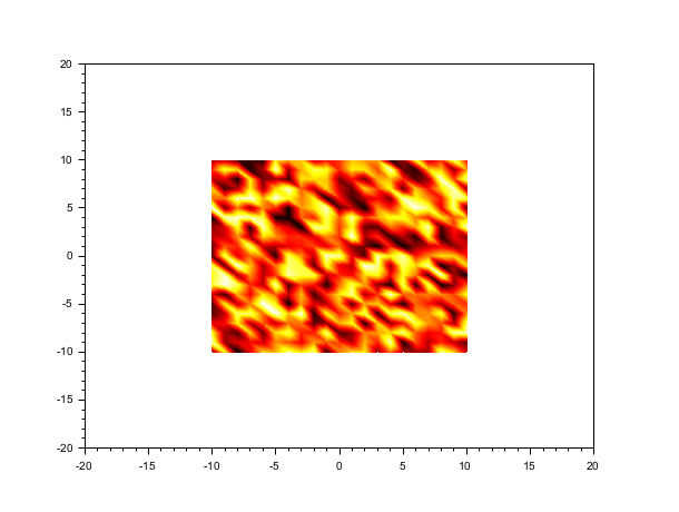
// example #1: rectangular grid
x = -10:10; y = -10:10; m = rand(21,21);
clf()
gcf().color_map = hot(64);
Sgrayplot(x, y, m, strf="011", rect=[-20,-20,20,20])
// example #2: rectangular grid with colorbar
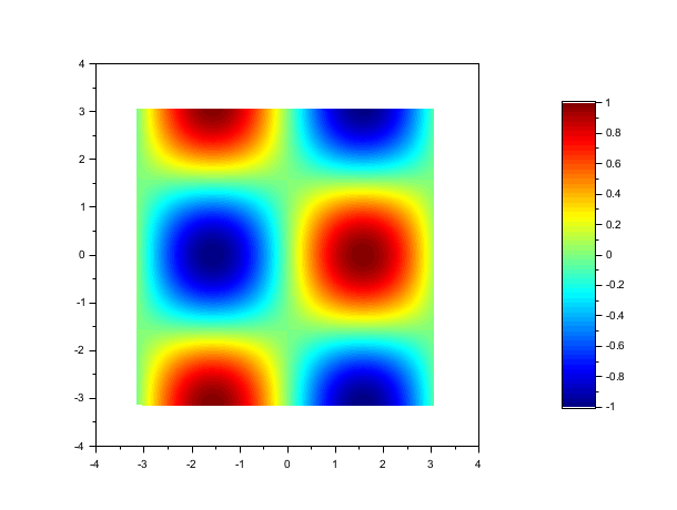
t = -%pi:0.1:%pi; m = sin(t)'*cos(t);
clf()
gcf().color_map = jet(64);
colorbar(-1,1)
Sgrayplot(t, t, m, strf="041")
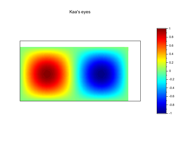
// example #3: animation — cos(t)*sin(x)*sin(y) on a rectangular grid
n = 30;
nt = 100;
x = linspace(0, 2*%pi, n);
y = linspace(0, %pi, n/2);
z = sin(x')*sin(y);
t = linspace(0, 4*%pi, nt);
show_window(); clf()
f = gcf();
f.color_map = jet(64);
colorbar(-1,1)
e = Sgrayplot(x, y, cos(t(1))*z, strf="042", zminmax=[-1,1])
xtitle("Kaa''s eyes")
for i = 1:nt
    e.data(:,3) = matrix(cos(t(i))*z, -1, 1);
end
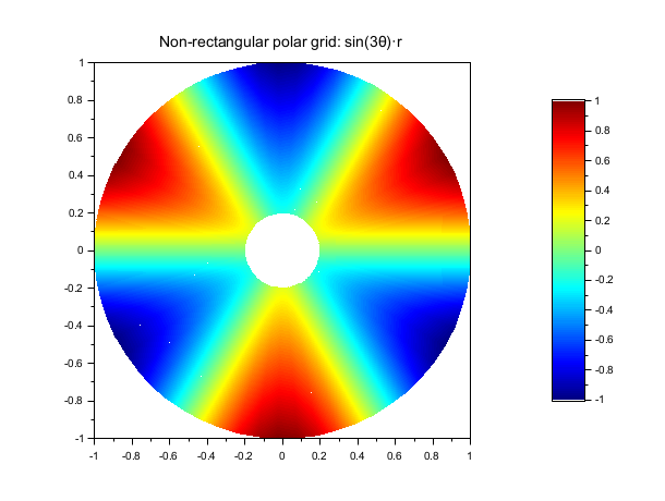
// example #4: non-rectangular (polar) grid
nr = 40; ntheta = 60;
r     = linspace(0.2, 1, nr);
theta = linspace(0, 2*%pi, ntheta);
[R, T] = ndgrid(r, theta);
X = R .* cos(T);
Y = R .* sin(T);
Z = sin(3*T) .* R;          // Z(i,j) = F(X(i,j), Y(i,j))
clf()
gcf().color_map = jet(128);
colorbar(-1,1)
Sgrayplot(X, Y, Z, strf="041")
xtitle("Non-rectangular polar grid: sin(3θ)·r")
See also
- fec — dessin en pseudo-couleurs d'une surface définie sur un maillage constitué de polygones convexes
- Sfgrayplot — smooth 2D plot of a surface defined by a function using colors
- fgrayplot — représentation 2D en pseudo-couleurs d'une surface définie par une fonction
- grayplot — 2D plot of a surface using colors
- colorbar — draws a vertical color bar
History
| Version | Description |
| 2025.0.0 | Function returns the created handle(s). |
| 2027.0.0 | Non-rectangular (curvilinear) grid support: X,Y,Z can now be matrices of the same size. |
| Report an issue | ||
| << Sfgrayplot | 2d_plot | stackedplot >> |