stackedplot
plot multiple timeseries on time axis
Syntax
stackedplot // demo
stackedplot(ts)
stackedplot(ts1, ..., tsN)
stackedplot(..., vars)
stackedplot(..., LineSpec)
stackedplot(..., LineSpec, GlobalProperty)
stackedplot(..., "CombineMatchingNames", %f)
stackedplot(..., Name, Value)
stackedplot(axes_handle, ...)
ax = stackedplot(..)
Arguments
- ts, ts1, ..., tsN
timeseries object
- vars
strings vector containing to variables names of timeseries
column index vector corresponding to position in variables names timeseries
cell of strings: each element can contain one or multiple variables names.
- LineSpec
This optional argument must be a string that will be used as a shortcut to specify a way of drawing a line. We can have one
LineSpecperyor{x,y}previously entered.LineSpecoptions deals with LineStyle, Marker and Color specifiers (see LineSpec). Those specifiers determine the line style, mark style and color of the plotted lines.- GlobalProperty
This optional argument represents a sequence of couple statements
{PropertyName,PropertyValue}that defines global objects properties applied to all the curves created by this plot. For a complete view of the available properties (see GlobalProperty).- Name, Value
'Title': string that contains the title of plot.
'DisplayLabels': matrix of strings that contains the names of Y-label for each axe. Default value: variables names of timeseries
'LegendLabels': matrix of strings that contains the names of timeseries.
- axes_handle
This optional argument forces the stackedplot to replace the axes given by
axes_handlerather than the current axes (see gca). Ifaxes_handlebelongs to a stackedplot, all the axes of this stackedplot are replaced.- ax
A vector of handle(s) to the axes created.
Description
The stackedplot function plots selected variables of one or more
timeseries objects in a set of vertically stacked axes
sharing the same time basis. All timeseries objects
passed to a single call must have the same time basis.
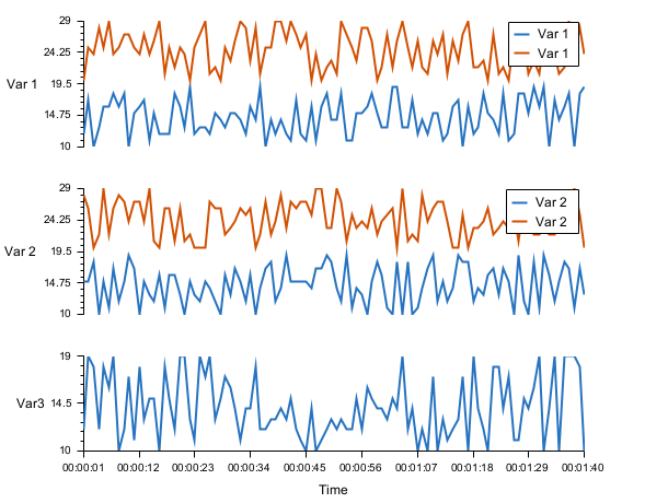
When two or more input timeseries have common variable
names, their curves are combined in the same graph by default.
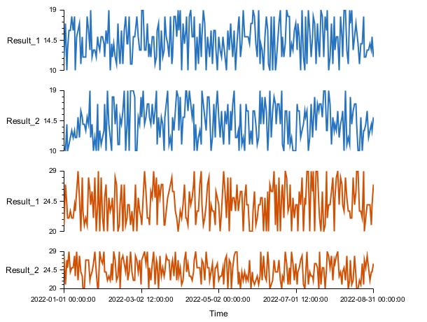
With "CombineMatchingNames", %f, a separate graph is
created for each variable of each timeseries.
Several independent stackedplot objects can be created
in the same figure. The stacked axes replace the current axes, so
stackedplot can be used after
subplot to build stacked plots in different
sub-regions of the same figure. Each axes created by stackedplot
is tagged "stackedplot:group:rank": when the current axes
belongs to a stacked plot, the whole stacked plot is replaced.
Axes belonging to another subplot are preserved.
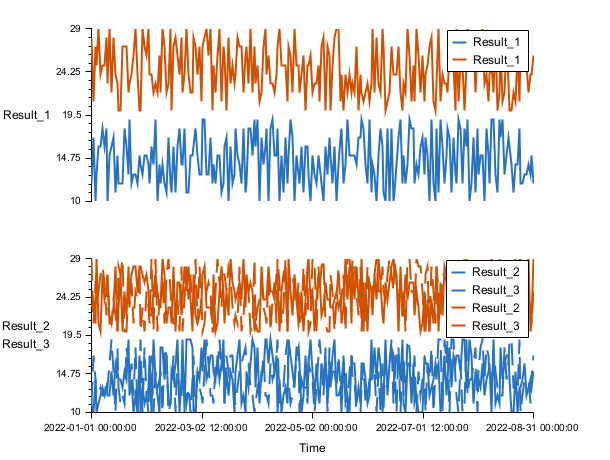
stackedplot(..., vars) plots only variables of timeseries specified by vars. vars can be
a vector of strings containing variables names to plot.
a vector of indexes corresponding to position of variables names in timeseries.
a cell containing variable names in matrices to plot them in same graphs. ie: {"var1", ["var2", "var3"]} will display var1 in a graph and var2 and var3 in another one.
stackedplot(..., LineSpec, GlobalProperty) customizes the line style, marker or color of polylines. This arguments are the same as the plot function.
stackedplot(..., "Title", str) adds a plot title.
stackedplot(..., "DisplayLabels", str) specifies the labels for the y-axis.
stackedplot(..., "LegendLabels", str) adds a legend for each plot. str is a vector of size N timeseries input. The legend can be used to specify the name of timeseries.
stackedplot(..., "CombineMatchingNames", %f) disables the default
grouping of variables having the same name across input
timeseries.
Enter the command stackedplot to see a demo.
Examples
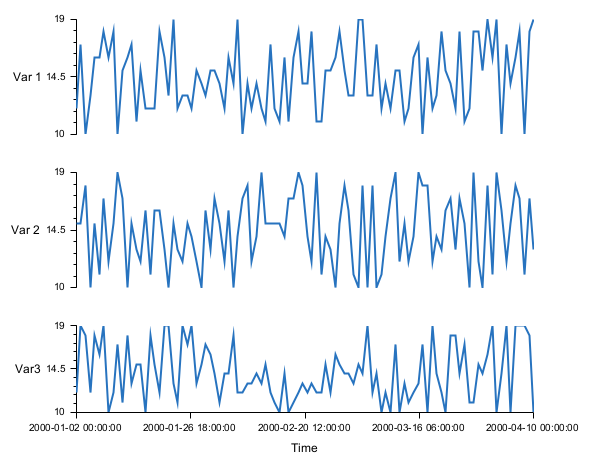
stackedplot(ts)
n = 100;
t = datetime(2000, 1, 1) + caldays(1:n)';
y = floor(10 * rand(n, 3)) + 10;
ts = timeseries(t, y(:, 1), y(:, 2), y(:, 3), "VariableNames", ["Time", "Var 1", "Var 2", "Var3"]);
stackedplot(ts);
stackedplot(ts1, ts2)
n = 100;
t = seconds(1:n)';
y1 = floor(10 * rand(n, 3)) + 10;
ts1 = timeseries(t, y1(:, 1), y1(:, 2), y1(:, 3), "VariableNames", ["Time", "Var 1", "Var 2", "Var3"]);

y2 = floor(10 * rand(n, 2)) + 20;
ts2 = timeseries(t, y2(:, 1), y2(:, 2), "VariableNames", ["Time", "Var 1", "Var 2"]);
stackedplot(ts1, ts2);
stackedplot(ts1, ts2, "CombineMatchingNames", %f)
t = datetime(2022, 1, 1):datetime(2022, 8, 31);
n = size(t, "*");
y1 = floor(10 * rand(n, 2)) + 10;
ts1 = timeseries(t, y1(:, 1), y1(:, 2), "VariableNames", ["Time", "Result_1", "Result_2"]);

y2 = floor(10 * rand(n, 2)) + 20;
ts2 = timeseries(t, y2(:, 1), y2(:, 2), "VariableNames", ["Time", "Result_1", "Result_2"]);
stackedplot(ts1, ts2);
stackedplot(ts1, ts2, "CombineMatchingNames", %f);
stackedplot(ts1, ts2, vars)
t = datetime(2022, 1, 1):datetime(2022, 8, 31);
n = size(t, "*");
y1 = floor(10 * rand(n, 3)) + 10;
ts1 = timeseries(t, y1(:, 1), y1(:, 2), y1(:, 3), "VariableNames", ["Time", "Result_1", "Result_2", "Result_3"]);

y2 = floor(10 * rand(n, 3)) + 20;
ts2 = timeseries(t, y2(:, 1), y2(:, 2), y2(:, 3), "VariableNames", ["Time", "Result_1", "Result_2", "Result_3"]);
stackedplot(ts1, ts2, ["Result_1", "Result_3"]);

stackedplot(ts1, ts2, [1 3]);

stackedplot(ts1, ts2, {"Result_1", ["Result_2", "Result_3"]});
stackedplot(ts1, ts2, "LegendLabels", str, "DisplayLabels", str2)
t = datetime(2022, 1, 1):datetime(2022, 8, 31);
n = size(t, "*");
y1 = floor(10 * rand(n, 3)) + 10;
ts1 = timeseries(t, y1(:, 1), y1(:, 2), y1(:,3), "VariableNames", ["Time", "Result_1", "Result_2", "Result_3"]);

y2 = floor(10 * rand(n, 3)) + 20;
ts2 = timeseries(t, y2(:, 1), y2(:, 2), y2(:, 3), "VariableNames", ["Time", "Result_1", "Result_2", "Result_3"]);
stackedplot(ts1, ts2, {"Result_1", ["Result_2", "Result_3"]}, "LegendLabels", ["t1", "t2"], "DisplayLabels", ["res1", "res2 - res3"]);
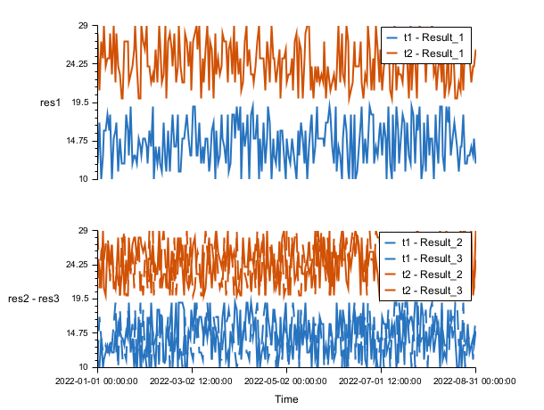
stackedplot with subplots
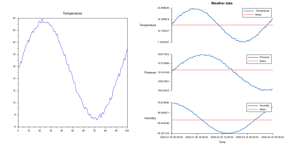
clf();
n = 100;
t = datetime(2020, 1, 1) + caldays(1:n)';

// Temperature, pressure and humidity
temperature = 15 + 8 * sin((1:n)' / 15) + rand(n, 1);
pressure = 1010 + 10 * sin((1:n)' / 20) + rand(n, 1);
humidity = 60 + 15 * cos((1:n)' / 18) + rand(n, 1);

ts = timeseries(t, temperature, pressure, humidity, ..
    "VariableNames", ["Time", "Temperature", "Pressure", "Humidity"]);
f = gcf();
f.axes_size = [1200; 600];
subplot(1, 2, 1);
plot(1:n, temperature);
title("Temperature");

subplot(1, 2, 2);
a = stackedplot(ts, "Title", "Weather data");
mean_values = [mean(humidity), mean(pressure), mean(temperature)];
x = gce().children.data(:,1);
x_ticks = gca().x_ticks;
for i = 3:-1:1
    plot(a(i), x, mean_values(i) * ones(1,n), "r");
    legend([ts.Properties.VariableNames(3-i+2); "Mean"])
    if i == 1 then
        a(i).x_ticks = x_ticks;
    else
        a(i).axes_visible(1) = "off";
    end
end
See also
- timeseries — create a timeseries - table with time as index
- subplot — grids the current figure or frame, and sets the current axes to a chosen cell
History
| Version | Description |
| 2027.0.0 |
Add The function now returns the handles of the created axes. |
| 2024.0.0 | Introduction in Scilab. |
| Report an issue | ||
| << semilogy | 2d_plot | 3d_plot >> |