Sfgrayplot
smooth 2D plot of a surface defined by a function using colors
Syntax
Sfgrayplot(x, y, f, <opt_args>)
Sfgrayplot(x, y, f [,strf, rect, nax, zminmax, colminmax, mesh, colout])
h = Sfgrayplot(...)
Arguments
- x, y
Real matrices defining the grid :
xandycan be row vectors of sizes n1 and n2 or matrices of the same size (n1,n2) (curvilinear grid).- f
a Scilab function of two variables.
Rectangular grid:
fis called asz(i,j) = f(x(i), y(j))viafeval(x, y, f); it receives scalar arguments and must return a scalar.Non-rectangular grid:
fis called asZ = f(X, Y)whereXandYare full matrices; it must return a matrix of the same size(n, m). The function should therefore be vectorized, using element-wise operators (.*, ./, .^, etc.).
- <opt_args>
this represents a sequence of statements
key1=value1, key2=value2, ...wherekey1,key2, ... can be one of the following:strf,rect,nax,zminmax,colminmax,mesh,colout(see plot2d for the first three and fec for the last four).- strf, rect, nax
see plot2d.
- zminmax, colminmax, mesh, colout
see fec.
- h
Optional output handle to the created
Fecentity. For a list of properties, see fec_properties.
Description
Sfgrayplot is the same as fgrayplot but
the plot is smoothed. The function fec is used for smoothing.
The surface is plotted assuming that it is linear on a set of triangles built
from the grid (here with n1=5, n2=3):
_____________
| /| /| /| /|
|/_|/_|/_|/_|
| /| /| /| /|
|/_|/_|/_|/_|
Two calling modes are available:
Rectangular grid:
Sfgrayplot(x, y, f)wherexandyare vectors. The functionfis evaluated on the full Cartesian product ofxandyusingfeval(x, y, f), sofreceives scalar arguments.Non-rectangular (curvilinear) grid:
Sfgrayplot(X, Y, f)whereXandYare matrices of the same size(n, m). The function is evaluated asZ = f(X, Y), sofmust be vectorized (accepting and returning matrices). This form is selected automatically when at least one of the first two arguments has more than one row and more than one column.
In both modes the grid is triangulated the same way: each quad
(i,j)-(i+1,j)-(i,j+1)-(i+1,j+1) is split into two
triangles along the diagonal, and fec interpolates
the computed Z values linearly inside each triangle.
The function colorbar may be used to see the color scale (but you must know or compute the min and max values of the surface).
Instead of Sfgrayplot, you can use
Sgrayplot when the Z values
are already available, and this may be slightly faster.
Enter the command Sfgrayplot() to see a demo.
Examples
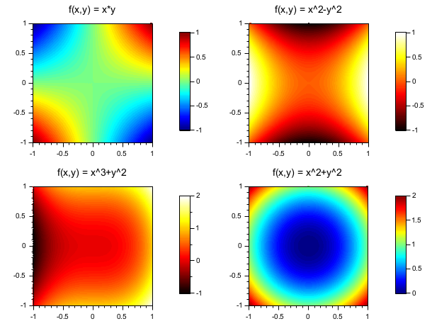
// example #1: rectangular grid — plot 4 surfaces
function z=surf1(x, y), z=x*y, endfunction
function z=surf2(x, y), z=x^2-y^2, endfunction
function z=surf3(x, y), z=x^3+y^2, endfunction
function z=surf4(x, y), z=x^2+y^2, endfunction
clf()
set(gcf(),"color_map",[jet(64);hot(64)])
x = linspace(-1,1,60);
y = linspace(-1,1,60);
drawlater();
subplot(2,2,1)
  colorbar(-1,1,[1,64])
  Sfgrayplot(x,y,surf1,strf="041",colminmax=[1,64])
  xtitle("f(x,y) = x*y")
subplot(2,2,2)
  colorbar(-1,1,[65,128])
  Sfgrayplot(x,y,surf2,strf="041",colminmax=[65,128])
  xtitle("f(x,y) = x^2-y^2")
subplot(2,2,3)
  colorbar(-1,2,[65,128])
  Sfgrayplot(x,y,surf3,strf="041",colminmax=[65,128])
  xtitle("f(x,y) = x^3+y^2")
subplot(2,2,4)
  colorbar(0,2,[1,64])
  Sfgrayplot(x,y,surf4,strf="041",colminmax=[1,64])
  xtitle("f(x,y) = x^2+y^2")
drawnow();
show_window()
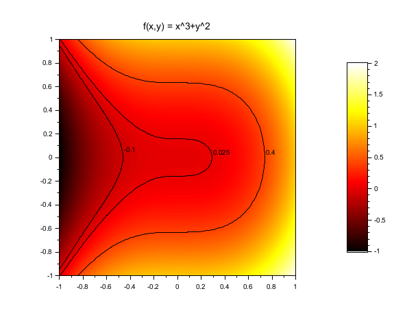
// example #2: rectangular grid — surf3 with contour lines
function z=surf3(x, y), z=x^3+y^2, endfunction
clf()
x = linspace(-1,1,60);
y = linspace(-1,1,60);
set(gcf(),"color_map",hot(128))
drawlater();
colorbar(-1,2)
Sfgrayplot(x,y,surf3,strf="041")
contour2d(x,y,surf3,[-0.1, 0.025, 0.4],style=[1 1 1],strf="000")
xtitle("f(x,y) = x^3+y^2")
drawnow();
show_window()
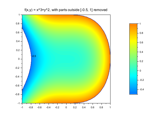
// example #3: rectangular grid — zminmax and colout optional arguments
//             restrict the plot to -0.5 <= z <= 1
function z=surf3(x, y), z=x^3+y^2, endfunction
clf()
x = linspace(-1,1,60);
y = linspace(-1,1,60);
set(gcf(),"color_map",jet(128))
drawlater();
zminmax = [-0.5 1]; colors=[32 96];
colorbar(zminmax(1),zminmax(2),colors)
Sfgrayplot(x, y, surf3, strf="041", zminmax=zminmax, colout=[0 0], colminmax=colors)
contour2d(x,y,surf3,[-0.5, 1],style=[1 1 1],strf="000")
xtitle("f(x,y) = x^3+y^2, with parts outside [-0.5, 1] removed")
drawnow();
show_window()
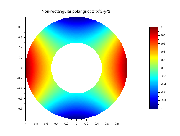
// example #4: non-rectangular (polar) grid
function Z=saddle(X, Y)
    Z = X.^2-Y.^2;
endfunction

nr = 40; ntheta = 80;
r     = linspace(0.5, 1, nr);
theta = linspace(0, 2*%pi, ntheta);
[R, T] = ndgrid(r, theta);
X = R .* cos(T);
Y = R .* sin(T);

clf()
gcf().color_map = jet(128);
colorbar(-1,1)
Sfgrayplot(X, Y, saddle, strf="041")
xtitle("Non-rectangular polar grid: z=x^2-y^2")
See also
History
| Version | Description |
| 2025.0.0 | Function returns the created handle(s). |
| 2027.0.0 | Non-rectangular (curvilinear) grid support: X,Y,Z can now be matrices of the same size. |
| Report an issue | ||
| << Matplot properties | 2d_plot | Sgrayplot >> |