cutaxes
plots curves or an existing axes along a discontinuous or multiscaled axis
Syntax
cutaxes(x, y, cutaxis, intervals)
cutaxes(axes0, cutaxis, intervals)
cutaxes(.., "ticksmode", "alt" | "shift")
cutaxes(.., "widths", "isoscaled" | widths)
[Axes, curves] = cutaxes(x, y, ..)
Axes = cutaxes(axes0, cutaxis, intervals, ..)
Contents
Arguments
- x
vector or matrix of real abscissae of curves to plot.
- If
xandyare vectors, we must havelength(x)==length(y) - If it is a vector and
yis a matrix, the same abscissae are shared for all curves given asycolumns, and we must havelength(x)==size(y,1). - If both
xandyare matrices, they must have the same sizes, andx(:,i)are abscissae ofy(:,i).
- If
- y
real numbers: ordinates of curves to plot. If
yis a matrix, each of its columns represents a separate curve.- axes0
Input graphical axes to replot in a piecewise way.
.isoview="off"is forced for all its piecewise replicates.- cutaxis
"x"or"y", specifying the discontinuous graphical axis.- intervals
(N x 2) matrix of real numbers: Each row provides both
[start,end]bounds of an interval over which all given curves or the inputaxes0must be plotted. According to thecutaxisvalue, given bounds are along the X axis or along the Y one. Any number of intervals may be specified as distinctintervalsrows.On the figure, intervals are plotted from left to right in the order they are specified in
intervals. The user may organize and present them as wished.When an interval is specified such that
start > end, the axis is reversed on the interval.- "ticksmode"
By default, ticks and labels of the different parts of the discontinuous axis are drawn "aligned", without specific attribute to distinguish consecutive parts.
"ticksmode"is an optional flag allowing to manage ticking and labelling of alternate pieces of the cut axis. It must be followed by one of the following values:"alt"Ticks and labels are drawn alternately on the bottom and top sides for the "x"discontinuous axis, or on the left and right sides for the"y"one."shift"Ticks and labels are drawn with a small alternative shift for one interval over two of the discontinuous axis. - "widths"
By default, if N intervals are defined, the full plot width is split into N sections of equal widths, whatever are the
|end - start|data ranges. This default plotting mode may be changed using the"widths"keyword, followed by one of the following specifications:"-"As the default mode, except that interspaces separating sections are removed. "isoscaled"This mode plots data with the same scale for all intervals along the discontinuous axis. The plotting width is proportional to the |end - start|range."-isoscaled"will do the same, except that interspaces separating sections are removed.widthsVector of numbers giving the relative graphical widths of intervals along the discontinuous axis. The vector must have as many values as there are defined intervals.
To remove the separating space before an interval, set its width as negative. Its absolute value will be used for the actual width.
Only
|widths| / sum(|widths|)is considered, in such a way that[1,2,2]and[0.5,1,1]or[0.2,0.4,0.4]are for instance equivalent.- Axes
vector of pointers on plotted sub-axes. The components allow to modify subaxes attributes, like the log mode of the piece of discontinuous axis, the grids, etc. See examples for illustrations.
Axes($)points to the common continuous axes.cutaxes()sets it as the current axes before returning.- curves
list of vectors of pointers on plotted curves (only when they are provided):
curves(i)is a vector of graphic pointers on all sections drawn for the curve #i defined iny(:,i).curves(i)(j)points to the section #j drawn for the curve #i overintervals(j,:).
These identifiers allow to modify curves attributes after plotting. For instance, setting in red all pieces of the curve #2 will be done with
curves(2).foreground = color("red"). Setting only its section #3 in dash style is done withcurves(2)(3).line_style = 3. An example is given and illustrated below. The vector of handles of curves #i1 to #i2 > #i1 of the same section #s may be retrieved with
Axes(s).children($).children($-i1+1:-1:$-i2+1).
Description
cutaxes() allows to plot some curves along a non-regular axis,
like having some hidden intervals. Consecutive visible intervals are drawn without
loosing space in-between.
When an input axes axes0 is provided instead of curves, it is
replicated as many times as there are intervals, each copy showing the axes contents over
an interval. The X, Y, and Z labels as well as the title of axes0
are ignored.
In both cases, cutaxes() draws in the gca() plotting area.
If axes0 is gca(), cutaxes()
deletes it before returning. Otherwise, axes0 is kept in its own
graphical area.
The intervals of the discontinous axis may have distinct scales, distinct linear or logarithmic modes, distinct direct or reversed modes.
A symetrical axis may be plotted by repeating an interval along the discontinuous axis and reverting the clone. See examples.
| cutaxes() can be used in conjunction to the following features:
|
Titles, legends and datatips
cutaxes() from an initial axes0:
The general title and the labels of the x and y axis are copied from the initial
axes0. If any, datatips are also copied. However, a given datatip
can't be dragged from an interval of the plot to other ones.
cutaxes(x,y,..) of some given curves, from scratch:
General title, title of the continuous common axis:
title(), xtitle(),
xlabel() when cutaxis is "y" or
ylabel() when cutaxis is "x"
can be used as usual after calling cutaxes().
Title of the discontinuous axis: It is highly
recommended to set a title to the axis of the most central plotted section,
rather than to the axis of the overall axes (which introduces a parasitic shift).
The handle of the targeted section will be used in conjunction to
xlabel() or ylabel(). Please see examples.
Datatips: can be set as usual on curves drawn with
cutaxes(). However, a given datatip can't be dragged from an
interval of the plot to other ones.
Block of curves legends: Such a block can be defined in a given plotting interval, by targeting the related axes:
sca(axes(i));
legend(["Curve 1" "Curve 2"],"in_upper_left");
Examples
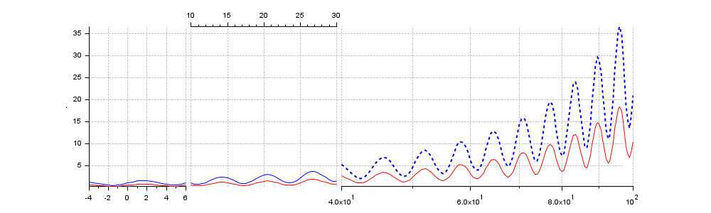
"ticksmode" and "widths" options. Addressing and customizing the curves
x = [-7.5:0.5:200]';
y =  exp(x/30).*(1+0.5*sin(x));

gcf().axes_size = [1000 300];
clf

intervals = [-4 6; 10 30 ; 40 100];
[a, c] = cutaxes(x, [y y/2], "x", intervals, "ticksmode", "alt", "widths", [1 1.5 3]);

// Special curves settings:
c(2).foreground = color("red");   // 2nd cuve in red
c1 = c(1);
c1(3).line_style = 8;             // 3rd section of 1st curve in small dashes
c1(3).thickness = 2;              //    .. and thicker

// Invert the common Y axis
//a.axes_reverse = ["off" "on"];

// Setting X-axis of the third section in log:
a(3).log_flags = "lnn";
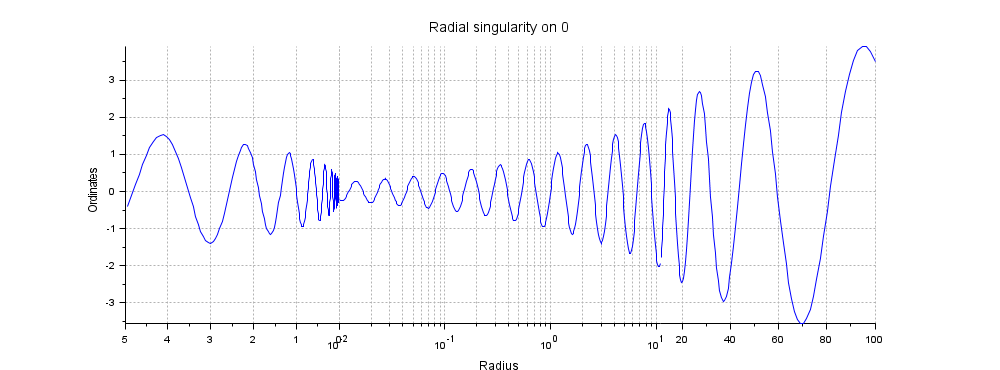
Replicated and inverted interval
cutaxes() allows to specify overlaying intervals, or the same interval
several times, or twice the same but in reverse order. This may be useful in various
situations. For a positive radial coordinate, it is thus possible to tick a
positive distance from the center on both sides. A side can be plotted in radial linear scale,
and the other in radial logarithmic scale to show the asymptotical behavior:
x = logspace(-2,2,500)';
y = sin(10*log(x)).*(x.^0.3);

gcf().axes_size = [1000 370];
clf

intervals = [5 0 ; 0.01 11 ; 11 max(x)];
a = cutaxes(x, y, "x", intervals, "widths", -[2 3 2]);
a(2).log_flags = "lnn";
a(2).sub_ticks(1) = 8;
title "Radial singularity on 0"
ylabel Ordinates
xlabel(a(2), "Radius")
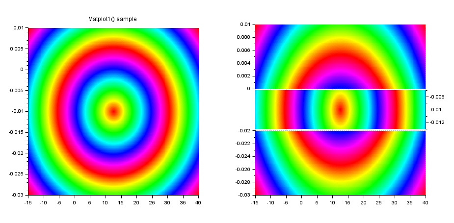
Multi-scaled Y axis:
Example #1, with curves legends:
x = [-8:0.2:100]';
y =  exp(x/14).*(1+0.5*sin(x));
intervals = [0.01 10 ; 10 max(y)];

gcf().axes_size = [1000 400];
clf
[a, c] = cutaxes(x, [y y/2], "y", intervals, "widths", -[1 2]);
c(2).foreground = color("red");
a(2).log_flags = "nln";
a(2).sub_ticks(2) = 8;
xlabel Abscissae
ylabel(a(2), "Ordinates") // a(2) is now the current axes
legend(["Curve 1" "Curve 2"], "in_upper_left");
// Grids
// a($).grid(1) = -1;       // removes the vertical shared grid
// a(1:$-1).grid(:,2)= -1;  // removes the horizontal grids

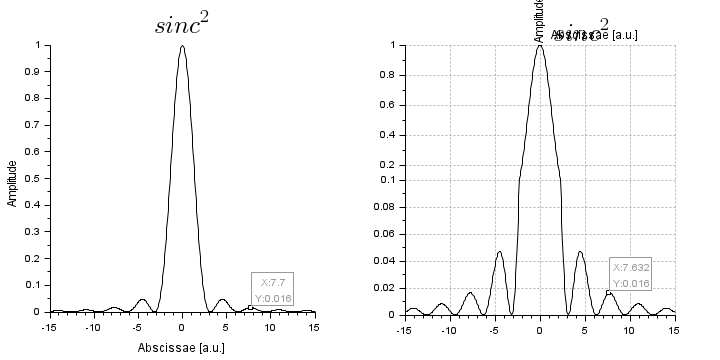
Example #2, from an axes: Low sinc2() bouncing wings
Here below we plot the curve to create its initial axes in subplot(1,2,1).
Then we move gca() to subplot(1,2,2), and
we call cutaxes(..) :
x = linspace(-15,15,400);
clf
subplot(1,2,1)
gcf().axes_size = [720 360];
plot2d(x, sinc(x).^2)
ax0 = gca();

d = datatipCreate(gce().children, [7.7 0.02]);
xtitle("$\LARGE sinc^2$", "Abscissae [a.u.]", "Amplitude")
grey = color("grey60");
set(d, "mark_size",4, "foreground",grey, "font_foreground",grey, "orientation",8);

subplot(1,2,2)
Axes = cutaxes(ax0, "y",[0 0.1 ; 0.1 1], "widths","-");
is_handle_valid(ax0)  // %T: the initial axes still exists
Now, gca() is kept where we have initially plotted the curve, and
we call cutaxes() to replicate it. As a consequence, cutaxes
uses the same subplot area, and finally deletes the initial axes after its replication:
x = linspace(-15,15,400);
clf
subplot(1,2,1)
gcf().axes_size = [720 360];
plot2d(x, sinc(x).^2)
ax0 = gca();
Axes = cutaxes(ax0, "y",[0 0.1 ; 0.1 1], "widths","-");
is_handle_valid(ax0)  // %F: the initial axes has been deleted

See Also
History
| Версия | Описание |
| 6.1.1 | Initial release in Scilab, proposed by S. Gougeon. cutaxes() was formerly named plotplots() and available as an ATOMS external module since 2018. |
| Report an issue | ||
| << contourf | 2d_plot | errbar >> |