colorbar
draws a vertical color bar
Syntax
colorbar
colorbar(umin, umax)
colorbar(umin, umax, colminmax)
colorbar(umin, umax, -1)
colorbar( , , [fmin fmax])
colorbar(.., Cformat)
Arguments
- Let U be the Z values of the plot for which a colorbar scale is needed, %inf, -%inf and %nan values being ignored.
- Let minU and maxU be the minimum and the maximum of U values.
- Let Nc be the Number of colors in the current color map:
Nc = size(gcf().color_map,1).
- umin
U's lowest data value covered by the colorbar.
Using
-%infsetsumin = min(U).When underlaying plotted data exist in the current axes,
uminmay be skipped -- using colorbar(,..) -- in order to extract and implicitly use min(U).- umax
U's biggest data value covered by the colorbar.
Using
%infsetsumax = max(U).When underlaying plotted data exist in the current axes,
umaxmay be skipped -- using colorbar(.., ,..) -- in order to extract and implicitly use max(U).- colminmax
implicit or explicit vector
[colmin, colmax]specifying the range of colors that span on the colorbar, corresponding to the[umin, umax]chosen data bounds.colminandcolmaxare indices of colors in the current colormap, with1 ≤ colmin < colmax ≤ Nc.Default setting:
[1,Nc]The dollar $ symbol can be used, standing for Nc. For example,
colminmax=[1 $/2]will use the first half of the colormap, andcolminmax=[$/2+1, $]will use the second half.Fractional bounds
[fmin, fmax]may also be specified, as well as using the special valuecolminmax=-1. Please see the description section for more details.- Cformat
word providing a C-format formatting the display of graduated values along the colorbar. The formatting syntaxes are described in the printf_conversion page.
Description
colorbar(…) draws a vertical color bar on the right side of
the current axes. The width of the targetted axes is priorly narrowed by 15%.
The freed room is used for the color bar, that is made of its own axes.
umin and umax set the data bounds scaling
the color bar at its bottom and top.
colminmax set the color range mapping the
[umin,umax] range, and used to fill the color bar.
When the current axes embeds an object of graphical type among
{"Matplot" "Fec" "Fac3d" "Plot3d" "Grayplot" "Champ"} and its related U data,
it is possible to skip umin or/and umax values.
min(U) or/and max(U) are then retrieved
from data and used to set the color bar. For a "Matplot" object, the case
.image_type=="index" is specifically processed.
 | Just after calling colorbar(…), gce() returns
the graphical handle of the color bar. |
The possible syntaxes are the following:
colorbar()
sets umin=minU and umax=maxU.
- For a Matplot.image_type="index", sets colminmax = [minU maxU].
- Otherwise, sets colminmax = [1 Nc]
colorbar(umin, umax, , Format)
sets colminmax=[1, Nc].
colorbar(umin, umax, -1)
sets colmin and colmax
such that "[colmin,colmax]/[1,Nc]" maps the "[umin,umax]/[minU,maxU]"
"ratio".
colorbar(,, [colmin colmax])
with integers such that 1 ≤ colmin < colmax ≤ Nc or using
$ standing for Nc.
Conversely to the previous one, this syntax sets
umin and umax
such that "[umin,umax]/[minU,maxU]" maps "[colmin,colmax]/[1,Nc]".
colorbar(,, [fmin fmax])
with 0 ≤ fmin < fmax ≤ 1, uses actual colors bounds
1+[fmin fmax]*(Nc-1), and uses proportional
umin and umax accordingly,
such that the relative range "[umin umax]/[min(U) max(U]" maps "[fmin, fmax]".
colorbar(-%inf, %inf, ..)
sets umin = minU, umax = maxU. Each one may be set to the U bound independently.
Examples
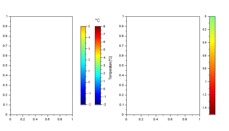
Example #1
Without underlaying U data : Direct umin and umax specifications.
clf reset                           // clears and resets the figure
gcf().color_map = jetcolormap(100); // sets its color map

// Axes on the left
// ----------------
subplot(1,2,1)                      // Now the default current axes
ax0 = gca();                        //  is on the half left
ax0.axes_bounds(3)  //  Here is its initial width

// The axes is clear. There is no plotted data.
// We explicitely create a colorbar from scratch:
colorbar(-2, 8, [1 100])    // It is inserted on the right

// The current (empty) axes is still the same:
gca() == ax0

// But its width has been shrunk (by -15%) to set the
// colorbar on its right side.
gca().axes_bounds

// gce() returns the handle of the color bar, to postprocess and customize it.
colbar1 = gce();
colbar1.type
ylabel(colbar1, "Temperature [°C]") // Let's add a label
title("°C")                         // or as title
colbar1.title.font_size = 3;        // .. with a bigger font
// Beware: xlabel(), ylabel() title() moves the focus to the bar.
sca(ax0); // Reset the focus to ax0 before going on

// Now plot a frame in the empty axes:
plot2d([], [], 0, "011", " ", [0 0 1 1])

// Then add some other color bars, still for the current axes
colorbar(-2, 5, [1 70])
// Set the labels in red
gce().font_color = color("red");

// The current axes is shrunk. The bar's width is decreased accordingly.

// axes on the right
// -----------------
subplot(1,2,2)
plot2d([], [], 0, "011", " ", [0 0 1 1])

ax1 = gca();
// top half of the colormap, with another data scale:
colorbar(0, 1.5, [$/2+1 $])

// Color bar post-processing
colbar3 = gce();
//      decrease its font size:
set(colbar3, "fractional_font","on","font_size", 0.5);
//      vertically extend the bar, to match the axes height:
colbar3.axes_bounds([2 4]) = ax1.axes_bounds([2 4]);
colbar3.margins([3 4]) = ax1.margins([3 4]);
//      reverse its graduations top-down:
colbar3.axes_reverse(2) = "on";
//      put its graduations on the left side:
colbar3.y_location = "left";

// Color bars are automatically redrawn and regraduated
// when resizing the figure. Try it!
➞ Customized color bar style:
--> ax0.axes_bounds(3)  //  Here is its initial width
 ans  =
   0.5

--> ...
--> // The current (empty) axes is still the same:
--> gca() == ax0
 ans  =
  T

--> ...
--> // But its width has been shrunk (by -15%) ...
--> gca().axes_bounds
 ans  =
   0.   0.   0.425   1.

--> ...
--> // gce() returns the handle of the color bar
--> colbar1 = gce();
--> colbar1.type
 ans  =
 Axes

--> colbar1 == gcf().children(1) // Another way to retrieve the handle
 ans  =
  T
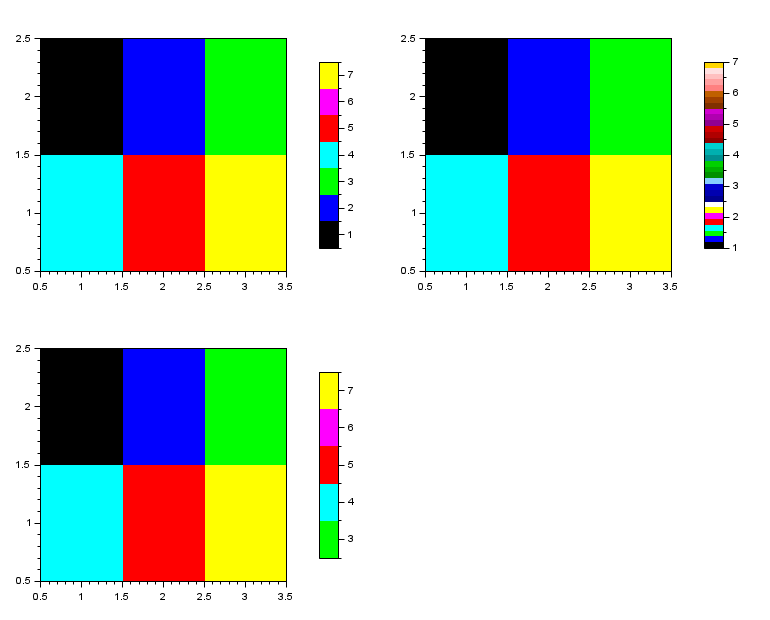
Example #2 : Matplot
After Matplot() here used with the default colormap.
clf reset   // Default colormap used
// 1) Matplot: implicit minU, maxU, colminmax = [umin umax]
subplot(2,2,1)
Matplot([1 2 3; 4 5 7]);
colorbar   // [1 7] graduations covered by colors #[1 7].
           // Ticks on middles of colored blocks

// 2) Matplot: Default colminmax = [1 Nc]
subplot(2,2,2)
Matplot([1 2 3;4 5 7]);
colorbar(1,7)   // [1 7] covered with the whole colormap.
                // "1" at the very bottom. "7" at the very top.

// 3) Matplot: another colors range, with explicit colminmax
subplot(2,2,3)
Matplot([1 2 3;4 5 7])
colorbar(3,7, [3 7])
// Ticks 2.5-7.5 expected:
//  - integer values ticked at the middle of colors blocks
//  - other .5 values ticked at the blocks separations
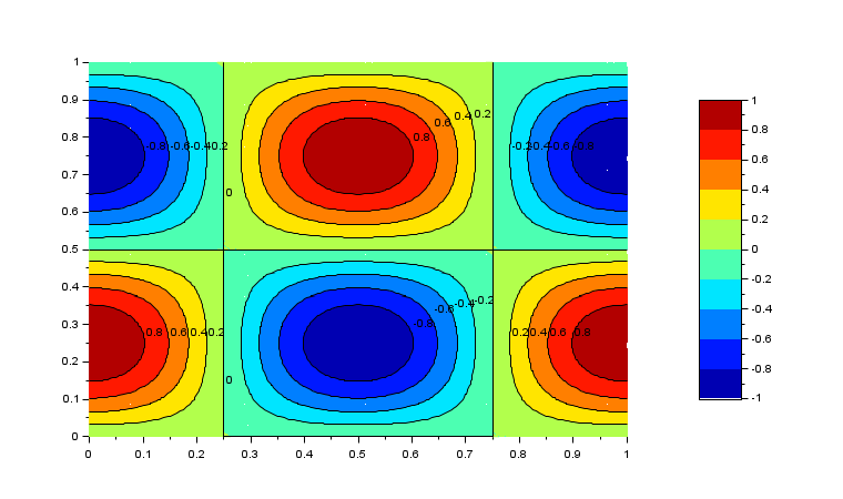
Example #3: After Sgrayplot()
U data are available from the underlaying Fec object.
Then umin and umax may be implicit.
Here we use a small number of colors, showing that a given [umin umax] data
range (here implicitly [-1, 1], is exactly covered by chosen colors.
x = linspace(0,1,81);
z = cos(2*%pi*x)'*sin(2*%pi*x);
n = 10;
clf
gcf().color_map = jetcolormap(n);
Sgrayplot(x, x, z);
contour(x,x,z,[-0.8 -0.6 -0.4 -0.2 0 0.2 0.4 0.6 0.8]);
gce().children.children(1:2:$-1).foreground=-1; // contours in black

colorbar
// Default umin = minU, umax = maxU, colminmax = [1 Nc]
// * "-1" tick at the very bottom of the scale
// * "1" tick at the very top
// * Nice subticks, at blocks middles & blocks limits
// * The contours levels must be at the right levels on the color bar
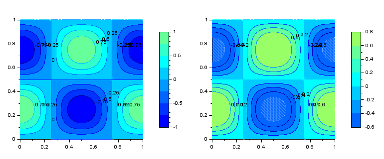
Partial colors range: 8 colors used over 20:
x = linspace(0,1,81);
z = cos(2*%pi*x)'*sin(2*%pi*x);
n = 8;
clf reset
gcf().color_map = jetcolormap(20);
gcf().axes_size = [770 320];

// 3.2) umin=minU and umax=maxU, covered by a subrange of colors
subplot(1,2,1)
Sgrayplot(x, x, z,colminmax=[3 n+2]);
contour(x,x,z,[-0.75 -0.5 -0.25 0 0.25 0.5 0.75]);
colorbar(-%inf,%inf,[3 n+2]);
// * The contours levels must be at the right levels on the color bar

// 3.3) Explicit umin and umax, with saturation for z values out of [umin, umax]:
subplot(1,2,2)
Sgrayplot(x, x, z, zminmax = [-0.6 0.8], colminmax = [5 11]);
contour(x,x,z,[-0.6 -0.4 -0.2 0.2 0.4 0.6]);
colorbar(-0.6, 0.8,[5 11]);
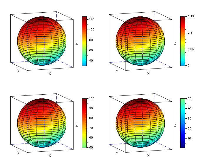
Example #4: for a Fac3d object
After plot3d1() or surf():
function [zz, zz1]=plotSphere()
    r = 0.3;
    orig = [1.5 0 0];
    deff("[x,y,z]=sph(alp,tet)",["x=r*cos(alp).*cos(tet)+orig(1)*ones(tet)";..
         "y=r*cos(alp).*sin(tet)+orig(2)*ones(tet)";..
         "z=r*sin(alp)+orig(3)*ones(tet)"]);
    [xx,yy,zz] = eval3dp(sph,linspace(-%pi/2,%pi/2,40),linspace(0,%pi*2,20));
    [xx1,yy1,zz1] = eval3dp(sph,linspace(-%pi/2,%pi/2,40),linspace(0,%pi*2,20));
    cc  = (xx+zz+2)*32;
    cc1 = (xx1-orig(1)+zz1/r+2)*32;
    plot3d1([xx xx1],[yy yy1],list([zz,zz1],[cc cc1]),theta=70,alpha=80,flag=[5,6,3])
endfunction

clf reset
gcf().color_map = jetcolormap(120);  // 120 colors available
gcf().axes_size = [670, 560];

// For these 4 plots of a sphere of radius 0.3,
//  the color-value relationship is the same.

// 3.0) Implicit min(u), max(u), on the whole color map
subplot(2,2,1)
plotSphere();
colorbar;               // graduations on [-0.3 0.3]

// 3.1) Selection of a data range. Color range set accordingly
subplot(2,2,2)
plotSphere();
colorbar(0.0, 0.15, -1);// graduations on [0, 0.15]

// 3.2) Selection of a colormap interval. umin & umax set accordingly
subplot(2,2,3)
plotSphere();
colorbar(,,[60 120]);  // graduations on [0, 0.3]

// 3.3) Selection of the first half of the colormap. umin & umax set accordingly
subplot(2,2,4)
plotSphere();
colorbar(,,[1 $/2]);  // graduations on [-0.3, 0]
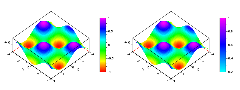
Example #5 : Plot3d object
After plot3d() or surf():
function plotSample()
    t=[-4:0.1:4];
    plot3d(t,t,sin(t)'*cos(t));
    e = gce();
    e.color_flag = 1;
    e.color_mode = -2;
endfunction

clf
gcf().color_map = rainbowcolormap(200);
gcf().axes_size = [800 300];

// 5.1) Bar graduated from minU=-1 to maxU=1 with the full colormap
subplot(1,2,1)
plotSample();
colorbar;

// 5.2) Consistent U/colors fractional selection (top 40%)
subplot(1,2,2)
plotSample();
colorbar(,,[0.6 1]);

gcf().children([2 4]).rotation_angles = [55 45];
Example #6: Demo
exec("SCI/modules/graphics/demos/colormap/colormaps.dem.sce",-1)
See also
History
| Версия | Описание |
| 6.0.2 |
|
| 6.1.0 |
|
| Report an issue | ||
| << color_list | color_management | colormap >> |