LSodar
LSodar (short for Livermore Solver for Ordinary Differential equations, with Automatic method switching for stiff and nonstiff problems, and with Root-finding) is a numerical solver providing an efficient and stable method to solve Ordinary Differential Equations (ODEs) Initial Value Problems.
Description
Called by xcos, LSodar (short for Livermore Solver for Ordinary Differential equations, with Automatic method switching for stiff and nonstiff problems, and with Root-finding) is a numerical solver providing an efficient and stable variable-size step method to solve Initial Value Problems of the form:

LSodar is similar to CVode in many ways:
- It uses variable-size steps,
- It can potentially use BDF and Adams integration methods,
- BDF and Adams being implicit stable methods, LSodar is suitable for stiff and nonstiff problems,
- They both look for roots over the integration interval.
The main difference though is that LSodar is fully automated, and chooses between BDF and Adams itself, by checking for stiffness at every step.
If the step is considered stiff, then BDF (with max order set to 5) is used and the Modified Newton method 'Chord' iteration is selected.
Otherwise, the program uses Adams integration (with max order set to 12) and Functional iterations.
The stiffness detection is done by step size attempts with both methods.
First, if we are in Adams mode and the order is greater than 5, then we assume the problem is nonstiff and proceed with Adams.
The first twenty steps use Adams / Functional method. Then LSodar computes the ideal step size of both methods. If the step size advantage is at least ratio = 5, then the current method switches (Adams / Functional to BDF / Chord Newton or vice versa).
After every switch, LSodar takes twenty steps, then starts comparing the step sizes at every step.
Such strategy induces a minor overhead computational cost if the problem stiffness is known, but is very effective on problems that require differentiate precision. For instance, discontinuities-sensitive problems.
Concerning precision, the two integration/iteration methods being close to CVode's, the results are very similar.
Examples
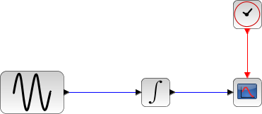

The integral block returns its continuous state, we can evaluate it with LSodar by running the example:
// Import the diagram and set the ending time
loadScicos();
loadXcosLibs();
importXcosDiagram("SCI/modules/xcos/examples/solvers/ODE_Example.zcos");
scs_m.props.tf = 5000;

// Select the LSodar solver
scs_m.props.tol(6) = 0;

// Start the timer, launch the simulation and display time
tic();
try xcos_simulate(scs_m, 4); catch disp(lasterror()); end
t = toc();
disp("Time for LSodar:", t);
The Scilab console displays:
Time for LSodar:
 9.546
Now, in the following script, we compare the time difference between LSodar and CVode by running the example with the five solvers in turn: Open the script
Time for LSodar:
 6.115

Time for BDF / Newton:
 18.894

Time for BDF / Functional:
 18.382

Time for Adams / Newton:
 10.368

Time for Adams / Functional:
 9.815
These results show that on a nonstiff problem, for the same precision required, LSodar is significantly faster. Other tests prove the proximity of the results. Indeed, we find that the solution difference order between LSodar and CVode is close to the order of the highest tolerance ( ylsodar - ycvode ≈ max(reltol, abstol) ).
Variable-size step ODE solvers are not appropriate for deterministic real-time applications because the computational overhead of taking a time step varies over the course of an application.
See also
- CVode — CVode (short for C-language Variable-coefficients ODE solver) is a numerical solver providing an efficient and stable method to solve Ordinary Differential Equations (ODEs) Initial Value Problems. It uses either BDF or Adams as implicit integration method, and Newton or Functional iterations.
- IDA — Implicit Differential Algebraic equations system solver, providing an efficient and stable method to solve Differential Algebraic Equations system (DAEs) Initial Value Problems.
- Runge-Kutta 4(5) — Runge-Kutta is a numerical solver providing an efficient explicit method to solve Ordinary Differential Equations (ODEs) Initial Value Problems.
- Dormand-Prince 4(5) — Dormand-Prince is a numerical solver providing an efficient explicit method to solve Ordinary Differential Equations (ODEs) Initial Value Problems.
- Implicit Runge-Kutta 4(5) — Numerical solver providing an efficient and stable implicit method to solve Ordinary Differential Equations (ODEs) Initial Value Problems.
- Crank-Nicolson 2(3) — Crank-Nicolson is a numerical solver based on the Runge-Kutta scheme providing an efficient and stable implicit method to solve Ordinary Differential Equations (ODEs) Initial Value Problems. Called by xcos.
- DDaskr — Double-precision Differential Algebraic equations system Solver with Krylov method and Rootfinding: numerical solver providing an efficient and stable method to solve Differential Algebraic Equations systems (DAEs) Initial Value Problems
- Comparisons — This page compares solvers to determine which one is best fitted for the studied problem.
- ode — программа решения обыкновенных дифференциальных уравнений
- ode_discrete — программа решения обыкновенных дифференциальных уравнений, моделирование дискретного времени
- ode_root — программа решения обыкновенных дифференциальных уравнений с поиском корней
- odedc — программа решения дискретно-непрерывных ОДУ
- impl — дифференциальное алгебраическое уравнение
Bibliography
ACM SIGNUM Newsletter, Volume 15, Issue 4, December 1980, Pages 10-11 LSode - LSodi
History
| Версия | Описание |
| 5.4.1 | LSodar solver added |
| Report an issue | ||
| << Solvers | Solvers | CVode >> |