scatter3d
3D scatter plot
Syntax
scatter3d()      // Example
scatter3d(x, y, z)
scatter3d(x, y, z, msizes)
scatter3d(x, y, z, msizes, mcolors)
scatter3d(.., "fill")
scatter3d(.., "fill", marker)
scatter3d(..., <marker_property, value>)
scatter3d(axes, ..)
polyline = scatter3d(..)
Arguments
- x, y, z
columns or rows vectors of n real numbers specifying the
x,yandzcoordinates of the centers of markers.- axes
- Handle of the graphical axes in which the scatter plot must be drawn. By default, the current axes is targeted.
- polyline
- Handle of the created polyline.
- msizes
Sizes of the markers, as of the area of the circle surrounding the marker, in point-square. Default value = 36. If it is scalar, the same size is used for all markers. Otherwise
msizesandxmust have the same number of elements.- mcolors
Colors of markers. If it is scalar, the same color is used for all markers. Otherwise,
mcolorsandxmust have the same number of elements.The same color is used for filling the body and drawing the edge of markers.
The values of
mcolorsare linearly mapped to the colors in the current colormap.A color can be specified by one of the following:
- Its name, among the predefined names colors (see the color_list).
- Its standard hexadecimal RGB code as a string, like "#A532FB".
- A matrix of RGB values with 3 columns and n rows, with Red Green and Blue intensities in [0,1].
- Its index in the current color map
- "fill"
By default, only the edge of markers is drawn, unless this keyword or the
"markerFaceColor"or"markerBackgroundColor"properties are set.- marker
Selects the shape of the markers. The same shape is used for all specified points. The figure below shows the 15 different marker shapes.
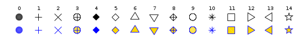
Each marker shape is specified either by its index (list above) or by its string symbol (table below).
Index String Marker type 0 "."Point 1 "+"Plus sign 2 "x"Cross 3 "circle plus"Circle with plus 4 "filled diamond"Filled diamond 5 "d"or"diamond"Diamond 6 "^"Upward-pointing triangle 7 "v"Downward-pointing triangle 8 "diamond plus"Diamond with plus 9 "o"Circle (default) 10 "*"Asterisk 11 "s"or"square"Square 12 ">"Right-pointing triangle 13 "<"Left-pointing triangle 14 "pentagram"or"p"Five-pointed star
Property <Name, Value> pairs
A series of property value pairs can be used to specify type, color and line width of the markers.
- "marker", value or "markerStyle", value
Shape of the marker (index or string keyword). See the table above.
- "markerEdgeColor", value or "markerForeground", value
Color of the edge of markers. Colors can be specified as for
mcolors. This option supersedesmcolors.- "markerFaceColor",value or "markerBackground",value
Color filling the body of markers. Colors can be specified as for
mcolors. This option supersedesmcolors.- "linewidth",value or "thickness",value
Specify the thickness of the edge for all markers. The unit for the value is one point.
Description
scatter3d(x,y,z) creates a scatter plot with markers at the locations
specified by x, y, and z.
The default type of the marker is a circle, the default color is "blue" and the default
marker size is 36.
This means the circle surrounding the marker has an area of 36 points squared.
Using scatter3d(x,y,z,s,c) different sizes and colors for each marker
can be specified.
There are many different ways to specify marker types, marker colors and marker sizes.
For more details see the description of the arguments and the examples.
 |
|
Examples
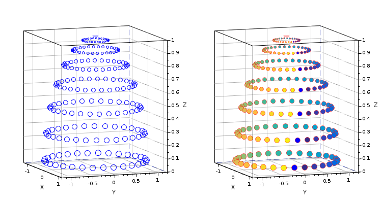
Create 3D scatter plot
// Data: points on an hemisphere
azimuth = 0:12:359;
latitude = 3:12:89;
[az, lat] = ndgrid(azimuth, latitude);
r = cosd(lat);
x = 1.1*cosd(az+lat/3) .* r;
y = 1.1*sind(az+lat/3) .* r;
z = sind(lat);

clf
gcf().color_map = parulacolormap(50);

subplot(1,2,1)    // Plot on the left
// Markers size according to r
scatter3d(x, y, z, r.^2*80);

subplot(1,2,2)    // Plot on the right
options = list("fill", "markerEdgeColor","red","thickness",0.5);
mcolors = az;     // + colors according to the azimuth
scatter3d(x, y, z, r.^2*80, mcolors, options(:));

// Tuning axes rendering
gcf().children.grid = [1 1 1]*color("grey50");
gcf().children.rotation_angles = [83 -20];
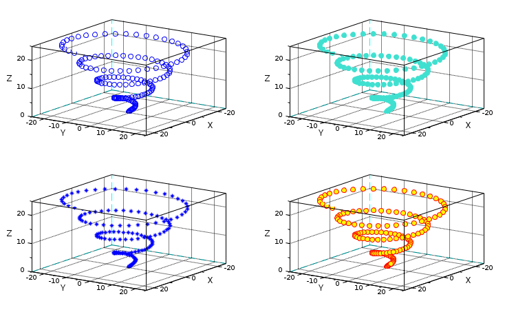
Styling the markers:
// Data
z = linspace(0, 25, 150);
x = z .* cos(z);
y = z .* sin(z);

subplot(2,2,1)
scatter3d(x, y, z)

// Fill the markers
subplot(2,2,2)
scatter3d(x, y, z, , "turquoise", "fill")

// Choose another marker shape
subplot(2,2,3)
scatter3d(x, y, z, "*");

// Customize the markers colors
subplot(2,2,4)
scatter3d(x, y, z,...
        "markerEdgeColor", [1 0 0],...
        "markerFaceColor", "yellow");

// Tune the 3D orientation of all axes
gcf().children.rotation_angles = [65 35];
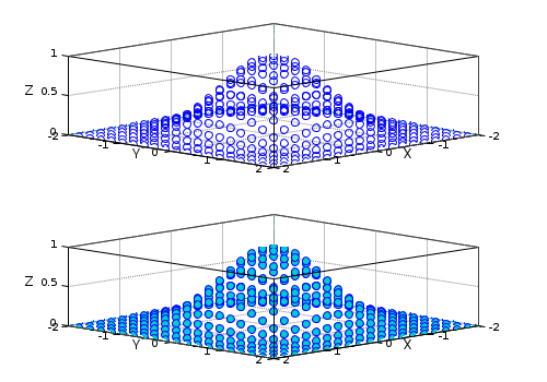
Specify subplot for scatter plot
// Data
n = 20;
[x, y] = meshgrid(linspace(-2, 2, n));
z = exp(-x.^2 - y.^2);

subplot(2,1,2)
axes2 = gca();
subplot(2,1,1)

scatter3d(x, y, z);
scatter3d(axes2, x(:), y(:), z(:), "markerFaceColor", [0 .8 .8]);

// Tune axes view
Axes = gcf().children;
Axes.rotation_angles = [60,45];
Axes.grid = [1 1 1]*color("grey50");
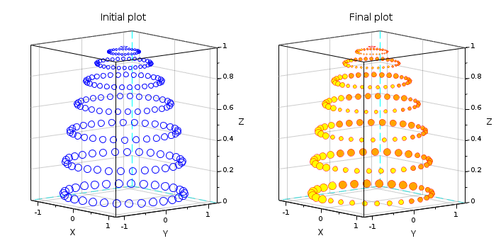
Use the handle to post-process the scatter plot:
// Data: points on an hemisphere
azimuth = 0:12:359;
latitude = 3:12:89;
[az, lat] = ndgrid(azimuth, latitude);
r = cosd(lat);
x = 1.1*cosd(az+lat/3) .* r;
y = 1.1*sind(az+lat/3) .* r;
z = sind(lat);

clf

subplot(1,2,1)
scatter3d(x, y, z, r.^2*80);
title("Initial plot", "fontsize",3)

subplot(1,2,2)
p = scatter3d(x, y, z, r.^2*80); // The same
title("Final plot", "fontsize",3)

// Let's post-process it through the handle:

// 1) Let's set all markers at y < 0 in yellow, and others in orange
np = size(p.data,1);  // number of points
tmp = ones(1,np) * color("orange");
tmp(p.data(:,2)<0) = color("yellow");
p.mark_background = tmp;

// 2) and markers at x > 0  1.4 smaller than other
tmp = p.data(:,1) > 0;
p.mark_size(tmp) = p.mark_size(tmp)/1.4;

// 3) Changing the edge color and thickness for all markers
p.mark_foreground = color("red");
p.thickness = 0.5;

// Tuning axes
Axes = gcf().children;
Axes.rotation_angles = [82, -40];
Axes.grid = [1 1 1]*color("grey60");
See also
- scatter — 2D scatter plot
- param3d — plots a single curve in a 3D cartesian frame
- gca — Return handle of current axes.
- gcf — Return handle of current graphic window.
- color_list — liste des noms de couleurs prédéfinies
- polyline_properties — description of the Polyline entity properties
History
| Version | Description |
| 6.0.0 | Function scatter3() introduced. |
| 6.1.0 | Function scatter3() set obsolete. scatter3d() is introduced. |
| 6.1.1 | Colors can be specified as well with their "#RRGGBB" hexadecimal standard code or their index in the color map. |
| Report an issue | ||
| << plot3d3 | 3d_plot | secto3d >> |