sprkode
SUNDIALS ordinary differential equation symplectic Runge-Kutta solver
Syntax
[t,y] = sprkode(f1,f2,tspan,y0,<opt_args>)
[t,y,info] = sprkode(f1,f2,tspan,y0,<opt_args>)
sol = sprkode(...)
solext = sprkode(sol,tfinal,<opt_args>)
sprkode(...)
Arguments
- f1, f2
a function, a string or a list, the right hand side(s) of the differential equation
- tspan
double vector, time interval or time points
- y0
a double array: initial state of the ode
- <opt_args>
a sequence of optional named arguments, see the solvers options
- t
vector of time points used by the solver
- y
array of solution at time values in
t- sol, solext
MList of
_odeSolutiontype, see the solution output help page- info
MList of
_odeSolutiontype with solver information, user events information (if applicable) and statistics- tfinal
final time of extended solution
Description
sprk computes the solution of Hamiltonian systems posed under the form


allowing for conservation of quadratic invariants (sprkode uses a symplectic integrator).
At the user level, when the dimension of the generalized momentum  and coordinates
  is n then
the right hand side functions
is n then
the right hand side functions f1(t,y) and f2(t,y) are called with a vector
of size 2*n and the partition of y is arbitrary chosen by the user when defining the initial conditions.
Then in the output of f1 the components of  must be set to zero, as well as the
the components of
must be set to zero, as well as the
the components of  output of
 f2 (see the example below).
As time adaptivity destroys the conservation properties, this solver must be used with a fixed step, hence the sequence of options
must set the fixedStep option.
As sprkode shares with arkode most of its features (syntax, specification of user functions) please refer to the Description section of arkode help page for basic usage (events handling, solution output, callback).
Example
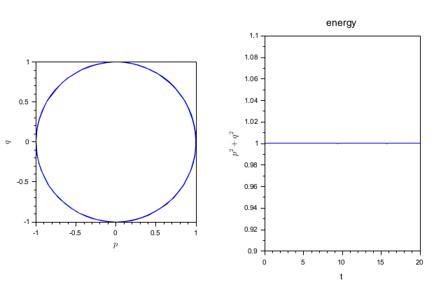
In the following example, we solve the harmonic oscilator Hamiltonian system.

function dpdt=f1(t, pq)
  q = pq(2);
  dpdt = [-q; 0];
end
function dqdt=f2(t, pq)
  p = pq(1);
  dqdt = [0; p]
end

[t,pq] = sprkode(f1,f2, [0 20], [1;0], fixedStep = 0.1)

subplot(1,2,1)
plot(pq(1,:),pq(2,:))
xlabel("$p$")
ylabel("$q$")
isoview("on")
subplot(1,2,2)
plot(t,sum(pq.^2,1))
gca().data_bounds(3:4) = [0.9,1.1];
xlabel("t")
ylabel("$p^2+q^2$")
title("energy")
Example
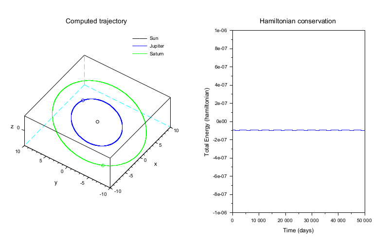
This second example solves a 3 body gravitationnal system (Sun, Supiter and Saturn)
function V=Ep(q)
    V(1) = - G*m0*m1/norm(q(sun)-q(jupiter)) - G*m0*m2/norm(q(sun)-q(saturn));
    V(2) = - G*m0*m1/norm(q(jupiter)-q(sun)) - G*m1*m2/norm(q(jupiter)-q(saturn));
    V(3) = - G*m0*m2/norm(q(saturn)-q(sun)) - G*m1*m2/norm(q(saturn)-q(jupiter));
endfunction

function K=Ec(p)
    K=[norm(p(sun))^2/(2*m0)
       norm(p(jupiter))^2/(2*m1)
       norm(p(saturn))^2/(2*m2)];
endfunction

function out=H(pq)
    nt = size(pq)(2)
    out = zeros(nt, 1)
    for i = 1:nt
        out(i) = sum(Ep(pq(10:$, i)) + Ec(pq(1:9, i)))
    end
endfunction

function dpdt=f1(t, pq)
   // Compute derivative of potentiel energy wrt. general position coordinates
   q = pq(10:$);
   dVdq(sun)     = -G*m0*m1*vecf(q(sun)-q(jupiter))..
                   -G*m0*m2*vecf(q(sun)-q(saturn));
   dVdq(jupiter) = -G*m1*m0*vecf(q(jupiter)-q(sun))..
                   -G*m1*m2*vecf(q(jupiter)-q(saturn));
   dVdq(saturn)  = -G*m2*m0*vecf(q(saturn)-q(sun))..
                   -G*m2*m1*vecf(q(saturn)-q(jupiter));
    dpdt = [dVdq; zeros(9,1)]
endfunction

function dqdt=f2(t, pq)
    p = pq(1:9);
    dTdp = [p(sun)/m0; p(jupiter)/m1; p(saturn)/m2];
    dqdt = [zeros(9,1); dTdp]
endfunction

vecf = #(v)->(v/norm(v).^3);

//  Initial positions and masses of three bodies relative to the sun
sun = 1:3;
jupiter = 4:6;
saturn = 7:9;
m0=1.00000597682;m1=9.54786104043e-4;m2=2.85583733151e-4;   // Relative masses to the sun
G=2.95912208286e-4;                                         // Gravitationnal constant
q0=[0;0;0; -3.5023653; -3.8169847; -1.5507963;..            // Positions expressed in Astronomical units
    9.0755314; -3.0458353; -1.6483708];
p0=[0;0;0;0.00565429*m1;-0.00412490*m1;-0.00190589*m1;..    // Initial impulse
    0.00168318*m2;0.00483525*m2;0.00192462*m2];

// Initial hamiltonian
H0 = sum(Ec(p0) + Ep(q0))

pq0 = [p0; q0]
h = 50;
tspan = 0:h:50000;

[_,pq] = sprkode(f1, f2, tspan, pq0, fixedStep = h)

Htot = H(pq)

q = pq(10:$, :)
q(jupiter,:) = q(jupiter,:)-q(sun,:);    // Frame reference shift to Solar frame
q(saturn,:) = q(saturn,:)-q(sun,:);
q(sun,:) = 0;

clf
subplot(1, 2, 2)
plot(tspan, Htot)
gca().data_bounds(3:4) = [-1e-6, 1e-6]
xlabel("Time (days)")
ylabel("Total Energy (hamiltonian)")
title("Hamiltonian conservation")
subplot(1, 2, 1)
title("Computed trajectory")

isoview on
comet3d(q([1 4 7],:)',q([2 5 8],:)',q([3 6 9],:)');
legend(gca().children([6 4 2]),["Sun"; "Jupiter"; "Saturn"],%f);
xlabel("x")
ylabel("y")
zlabel("z")
Available sprkode methods
| Method identifier | Order | Aliases |
| EULER_1_1 | 1 | SPRK_1 |
| LEAPFROG_2_2 | 2 | SPRK_2 |
| PSEUDO_LEAPFROG_2_2 | 2 | |
| MCLACHLAN_2_2 | 2 | |
| RUTH_3_3 | 3 | |
| MCLACHLAN_3_3 | 3 | SPRK_3 |
| MCLACHLAN_4_4 | 4 | SPRK_4 |
| CANDY_ROZMUS_4_4 | 4 | |
| MCLACHLAN_5_6 | 5 | SPRK_5 |
| YOSHIDA_6_8 | 6 | SPRK_6 |
| SUZUKI_UMENO_8_16 | 8 | SPRK_8 |
| SOFRONIOU_10_36 | 10 | SPRK_10 |
See also
- arkode — SUNDIALS ordinary differential equation additive Runge-Kutta solver
- cvode — SUNDIALS ordinary differential equation solver
- ida — SUNDIALS differential-algebraic equation solver
- User functions — Coding user functions used by SUNDIALS solvers
- Options (ODE and DAE solvers) — Changing the default behavior of solver
Bibliography
E. Hairer, C. Lubich, G. Wanner, "Structure-Preserving Algorithms for Ordinary Differential Equations", Springer Series in Computational Mathematics, 2006, https://doi.org/10.1007/3-540-30666-8
D. R. Reynolds, D. J. Gardner, C. S. Woodward and C. J. Balos, "User Documentation for arkode", 2026, v6.7.0, available online at https://sundials.readthedocs.io/en/latest/arkode.
| Report an issue | ||
| << kinsol | SUite of Nonlinear and DIfferential/ALgebraic equation - SUNDIALS solvers | bvode >> |