splin3d
spline gridded 3d interpolation
Syntax
tl = splin3d(x, y, z, v)
tl = splin3d(x, y, z, v, order)
Arguments
- x,y,z
strictly increasing row vectors (each with at least 3 components) defining the 3d interpolation grid
- v
nx x ny x nz hypermatrix (nx, ny, nz being the length of
x,yandz)- order
(optional) a 1x3 vector [kx,ky,kz] given the order of the tensor spline in each direction (default [4,4,4], i.e. tricubic spline)
- tl
a tlist of type splin3d defining the spline
Description
This function computes a 3d tensor spline s
which interpolates the (xi,yj,zk,vijk) points, ie, we
have s(xi,yj,zk)=vijk for all
i=1,..,nx, j=1,..,ny and
k=1,..,nz. The resulting spline
s is defined by tl which consists
in a B-spline-tensor representation of s. The
evaluation of s at some points must be done by the
interp3d function (to compute
s and its first derivatives) or by the
bsplin3val function (to compute an arbitrary
derivative of s) . Several kind of splines may be
computed by selecting the order of the spline in each direction
order=[kx,ky,kz].
Remark : This function works under the conditions
| nx, ny, nz ≥ 3 |
| 2 ≤ kx < nx |
| 2 ≤ ky < ny |
| 2 ≤ kz < nz |
An error is yielded when they are not respected.
Examples
// example 1
// =============================================================================

func =  "v=cos(2*%pi*x).*sin(2*%pi*y).*cos(2*%pi*z)";
deff("v=f(x,y,z)",func);
n = 10;  // n x n x n  interpolation points
x = linspace(0,1,n); y=x; z=x; // interpolation grid
[X,Y,Z] = ndgrid(x,y,z);
V = f(X,Y,Z);
tl = splin3d(x,y,z,V,[5 5 5]);
m = 10000;
// compute an approximated error
xp = grand(m,1,"def"); yp = grand(m,1,"def"); zp = grand(m,1,"def");
vp_exact = f(xp,yp,zp);
vp_interp = interp3d(xp,yp,zp, tl);
er = max(abs(vp_exact - vp_interp))
// now retry with n=20 and see the error
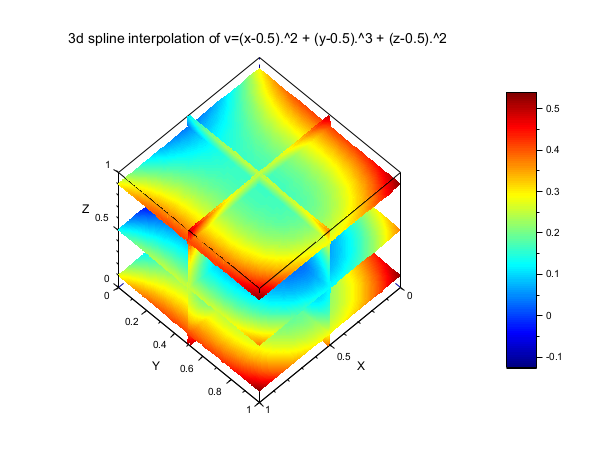
// example 2 (see linear_interpn help page which have the
//            same example with trilinear interpolation)
// =============================================================================

exec("SCI/modules/interpolation/demos/interp_demo.sci", -1);
func =  "v=(x-0.5).^2 + (y-0.5).^3 + (z-0.5).^2";
deff("v=f(x,y,z)",func);
n = 5;
x = linspace(0,1,n); y=x; z=x;
[X,Y,Z] = ndgrid(x,y,z);
V = f(X,Y,Z);
tl = splin3d(x,y,z,V);
// compute (and display) the 3d spline interpolant on some slices
m = 41;
direction = ["z="  "z="  "z="  "x="  "y="];
val = [ 0.1   0.5   0.9   0.5   0.5];
ebox = [0 1 0 1 0 1];
[XF, YF, ZF, VF] = ([], [], [], []);
for i = 1:length(val)
  [Xm,Xp,Ym,Yp,Zm,Zp] = slice_parallelepiped(direction(i), val(i), ebox, m, m, m);
  Vm = interp3d(Xm,Ym,Zm, tl);
  [xf,yf,zf,vf] = nf3dq(Xm,Ym,Zm,Vm,1);
  XF = [XF xf]; YF = [YF yf]; ZF = [ZF zf]; VF = [VF vf];
  Vp = interp3d(Xp,Yp,Zp, tl);
  [xf,yf,zf,vf] = nf3dq(Xp,Yp,Zp,Vp,1);
  XF = [XF xf]; YF = [YF yf]; ZF = [ZF zf]; VF = [VF vf];
end

clf
[nb_col, vmin, vmax] = (128, min(VF), max(VF));
color_example = dsearch(VF,linspace(vmin,vmax,nb_col+1));
gcf().color_map = jet(nb_col);
gca().hiddencolor = gca().background;
colorbar(vmin,vmax)
plot3d(XF, YF, list(ZF,color_example), flag=[-1 6 4])
title("3d spline interpolation of "+func, "fontsize",3)
See also
- linear_interpn — n dimensional linear interpolation
- interp3d — 3d spline evaluation function
- bsplin3val — 3d spline arbitrary derivative evaluation function
| Report an issue | ||
| << splin2d | Interpolation | Control Systems - CACSD >> |