polyfit
Polynomial curve fitting
Syntax
p = polyfit(x, y, n [,w])
[p, S] = polyfit(x, y, n [,w])
[p, S, mu] = polyfit(x, y, n [,w])
Arguments
- x
real or complex vector/matrix
- y
real or complex vector/matrix.
ymust have the same size asx- n
an integer, n>=0. It is a degree of the fitting polynomial. Or a polynom. In the case,
polyfitextracts the degree of polynom and returns a polynom containing the coefficients.- w
real vector/matrix, the weights to apply to each
yvalue. Default value: ones(x).- p
a
1xn+1real or complex vector or polynom, the polynomial coefficients- S
a structure containing the following fields:
- R
a matrix of doubles, the triangular factor R form the qr decomposition
- df
a real, the degrees of freedom
- normr
a real, the norm of the residuals
- mu
a
1x2vector.mu(1)ismean(x)andmu(2)isstdev(x)
Description
p = polyfit(x, y, n) returns a vector of coefficients of a polynomial p(x)
of degree n:

Depending on the type of n, p will be a real or complex vector or a polynom.
p can be used with polyval function to evaluate the polynomial at the data points.
[p, S] = polyfit(x, y, n) returns a vector of coefficients of a polynomial and a structure
S that can be used with polyval to compute the estimated error of the predicted values.
[p, S, mu] = polyfit(x, y, n) returns a third output argument mu
containing [mean(x), stdev(x)]. x is centered at zero and scaled to have unit standard deviation.
p = polyfit(x, y, n, w) specifies weights to apply to each y value.
Examples
Some examples use lambda functions.
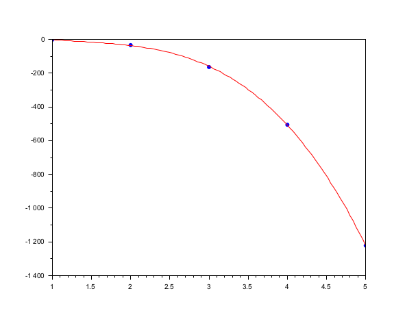
example 1 - p = polyfit(x, y, n)
x = 1:5;
// Use lambda function
y = #(x) -> (-2*x.^4 + x.^3 - 5 * x.^2 + 6 *x -2);
p = polyfit(x, y(x), 3)

xx = linspace(1, 5, 100);
yy = polyval(p, xx);

plot(x, y(x), "b.", "thickness", 2);
plot(xx, yy, "r");

example 2 - p = polyfit(x, y, n) with n a polynom
function r=y(x)
    r = -2*x.^4 + x.^3 - 5 * x.^2 + 6 *x -2;
endfunction

x = 1:5;
p = polyfit(x, y(x), %s^3)

xx = linspace(1, 5, 100);
yy = polyval(p, xx);

plot(x, y(x), "b.", "thickness", 2);
plot(xx, yy, "r");
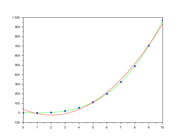
example 3 - [p, S, mu] = polyfit(x, y, n)
x = 0:10;
// Use lambda function
y = #(x) -> (x.^3 - 3*x + 2);

[p, S, mu] = polyfit(x, y(x), 2)

xx = linspace(0, 10, 100);
yy = polyval(p, xx, S, mu);

plot(x, y(x), "b.", "thickness", 2);
plot(xx, y(xx), "g");
plot(xx, yy, "r");
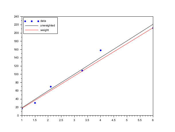
example 4 - p = polyfit(x, y, n, w)
x = [1 1.5 2.1 3.3 4 6];
y = 39 *x - [22 28 12 20 -2 22];
w = [1 0.25 0.11 0.8 0.2 1]

p = polyfit(x,y,1)
pw = polyfit(x,y,1,w)

xx = 1:6;
yy = polyval(p, xx); // unweighted
yyw = polyval(pw, xx); // weighted

plot(x, y, ".")
plot(xx, yy, "k")
plot(xx, yyw, "r")

legend(["data"; "unweighted"; "weight"], "in_upper_left")
History
| Version | Description |
| 2025.0.0 | Introduction in Scilab. |
| 2025.1.0 | Weights ( |
| Report an issue | ||
| << pdist2 | Statistics | polyval >> |