Please note that the recommended version of Scilab is 2026.1.0. This page might be outdated.
See the recommended documentation of this function
kpure
continuous SISO system limit feedback gain
Syntax
[K,R] = kpure(sys)
[K,R] = kpure(sys, tol)
Arguments
- sys
A SISO linear dynamical system, in state space, transfer function or zpk representations, in continuous or discrete time.
- tol
a positive scalar. tolerance used to determine if a root is imaginary or not. The default value is
1e-6- K
Real vector, the vector of gains for which at least one closed loop pole is imaginary.
- R
Complex vector, the imaginary closed loop poles associated with the values of
K.
Description
K=kpure(sys) computes the gains K such that the system
sys feedback by K(i) (sys/.K(i)) has poles on imaginary axis.
Examples
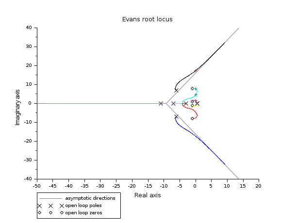
num=real(poly([-1+%i, -1-%i, -1+8*%i  -1-8*%i],'s'));
den=real(poly([0.5 0.5  -6+7*%i  -6-7*%i  -3 -7 -11],'s'));
h=num/den;

[K,Y]=kpure(h)
clf(); evans(h)
plot(real(Y),imag(Y),'+r')
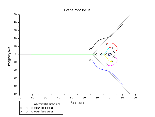
num=real(poly([-1+%i*1, -1-%i*1, 2+%i*8  2-%i*8 -2.5+%i*13 -2.5-%i*13],'s'));
den=real(poly([1 1 3+%i*3 3-%i*3 -15+%i*7  -15-%i*7  -3 -7 -11],'s'));
h=num/den;

[K,Y]=kpure(h)
clf(); evans(h,100000)
plot(real(Y),imag(Y),'+r')
History
| Version | Description |
| 6.0 | Handling zpk representation |
| Report an issue | ||
| << Placement de pôles | Placement de pôles | krac2 >> |