Please note that the recommended version of Scilab is 2026.0.1. This page might be outdated.
See the recommended documentation of this function
flts
time response (discrete time, sampled system)
Syntax
y = flts(u, sl)
y = flts(u, sl, past)
y = flts(u, sl, x0)
[y,x] = flts(u, sl, x0)
Arguments
- u
matrix (input vector)
- sl
A linear dynamical system, in state space, transfer function or zpk representations, in discrete time.
- x0
vector (initial state ; default value=
0)- past
matrix (of the past ; default value=
0)- x,y
matrices (state and output)
Description
State-space form:
sl is a discrete linear system given by its state
space representation (see syslin ):
sl=syslin('d',A,B,C,D) :
x[t+1] = A x[t] + B u[t]
y[t]   = C x[t] + D u[t]
or, more generally, if D is a polynomial matrix
(p = degree(D(z))) :
D(z) = D_0 + z D_1 + z^2 D_2 +..+ z^p D_p
y[t] = C x[t] + D_0 u[t] + D_1 u[t+1] +..+ D_[p] u[t+p]
Transfer form:
y=flts(u,sl[,past]). Here sl
is a linear system in transfer matrix representation i.e
sl=syslin('d',transfer_matrix) (see
syslin
).
past = [u     ,...,  u   ]
       [ -nd           -1]
       [y     ,...,  y   ]
       [ -nd           -1]
is the matrix of past values of u and y.
nd is the maximum of degrees of lcm's of each row
of the denominator matrix of sl.
u = [u0 u1 ... un]  (input)
y = [y0 y1 ... yn]  (output)
p is the difference between maximum degree of numerator and maximum degree of denominator
Examples
sl=syslin('d',1,1,1);u=1:10;
y=flts(u,sl);
plot2d(y)
[y1,x1]=flts(u(1:5),sl);y2=flts(u(6:10),sl,x1);
y-[y1,y2]

//With polynomial D:
z=poly(0,'z');
D=1+z+z^2; p =degree(D);
sl=syslin('d',1,1,1,D);
y=flts(u,sl);[y1,x1]=flts(u(1:5),sl);
y2=flts(u(5-p+1:10),sl,x1);  // (update)
y-[y1,y2]

//Delay (transfer form): flts(u,1/z)
// Usual responses
z=poly(0,'z');
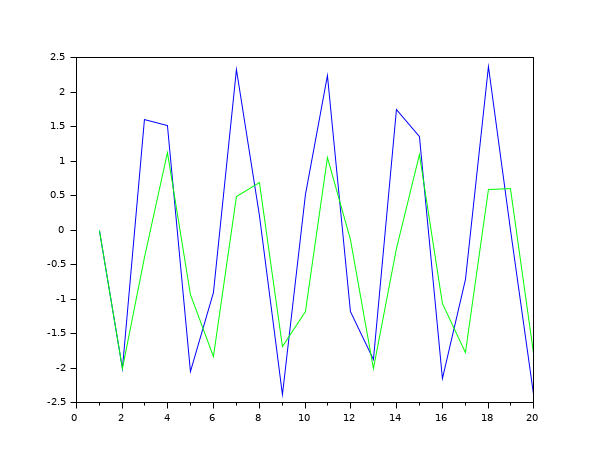
h=syslin(0.1,(1-2*z)/(z^2+0.3*z+1))
imprep=flts(eye(1,20),tf2ss(h));   //Impulse response
clf();
plot(imprep,'b')
u=ones(1,20);
stprep=flts(ones(1,20),tf2ss(h));   //Step response
plot(stprep,'g')

// Other examples
A=[1 2 3;0 2 4;0 0 1];
B=[1 0;0 0;0 1];
C=eye(3,3);
Sys=syslin('d',A,B,C);
H=ss2tf(Sys); u=[1;-1]*(1:10);
//
yh=flts(u,H); ys=flts(u,Sys);
norm(yh-ys,1)
//hot restart
[ys1,x]=flts(u(:,1:4),Sys);ys2=flts(u(:,5:10),Sys,x);
norm([ys1,ys2]-ys,1)
//
yh1=flts(u(:,1:4),H);yh2=flts(u(:,5:10),H,[u(:,2:4);yh(:,2:4)]);
norm([yh1,yh2]-yh,1)
//with D<>0
D=[-3 8;4 -0.5;2.2 0.9];
Sys=syslin('d',A,B,C,D);
H=ss2tf(Sys); u=[1;-1]*(1:10);
rh=flts(u,H); rs=flts(u,Sys);
norm(rh-rs,1)
//hot restart
[ys1,x]=flts(u(:,1:4),Sys);ys2=flts(u(:,5:10),Sys,x);
norm([ys1,ys2]-rs,1)
//With H:
yh1=flts(u(:,1:4),H);yh2=flts(u(:,5:10),H,[u(:,2:4); yh1(:,2:4)]);
norm([yh1,yh2]-rh)
See also
History
| Version | Description |
| 6.0 | handling zpk representation |
| Report an issue | ||
| << dsimul | Time Domain | ltitr >> |