Scilab 6.0.2
Please note that the recommended version of Scilab is 2026.1.0. This page might be outdated.
See the recommended documentation of this function
gainplot
magnitude plot
Syntax
gainplot(sl,fmin,fmax [,step] [,comments] )
gainplot(frq,db,phi [,comments])
gainplot(frq, repf [,comments])
Arguments
- sl
A siso or simo linear dynamical system, in state space, transfer function or zpk representations, in continuous or discrete time.
- fmin,fmax
real scalars (frequency interval).
- step
real (discretization step (logarithmic scale))
- comments
string
- frq
matrix (row by row frequencies)
- db,phi
matrices (magnitudes and phases corresponding to
frq)- repf
complex matrix. One row for each frequency response.
Description
Same as bode but plots only the magnitude.
Examples
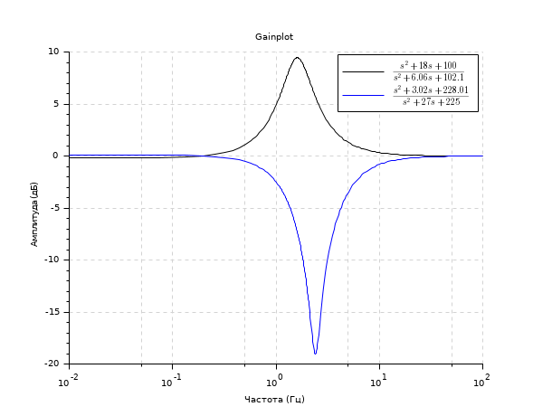
s=poly(0,'s')
h1=syslin('c',(s^2+2*0.9*10*s+100)/(s^2+2*0.3*10.1*s+102.01))
h2=syslin('c',(s^2+2*0.1*15.1*s+228.01)/(s^2+2*0.9*15*s+225))
clf();gainplot([h1;h2],0.01,100,..
                   ["$\frac{s^2+18 s+100}{s^2+6.06 s+102.1}$";
                    "$\frac{s^2+3.02 s+228.01}{s^2+27 s+225}$"])
title('Gainplot')
See also
History
| Версия | Описание |
| 6.0 | handling zpk representation |
| Report an issue | ||
| << freson | Frequency Domain | hallchart >> |