Please note that the recommended version of Scilab is 2026.1.0. This page might be outdated.
See the recommended documentation of this function
bvode
boundary value problems for ODE using collocation method
bvodeS
Simplified call to bvode
Syntax
zu = bvode(xpoints,N,m,x_low,x_up,zeta,ipar,ltol,tol,fixpnt,fsub,dfsub,gsub,dgsub,guess)
zu = bvodeS(xpoints,m,N,x_low,x_up,fsub,gsub,zeta, <optional_args>)
Arguments
- zu
a column vector of size
M. The solution of the ode evaluated on the mesh given by points. It containsz(u(x))for each requested points.- xpoints
an array which gives the points for which we want to observe the solution.
- N
a scalar with integer value, number of differential equations (
N<= 20).- m
a vector of size
Nwith integer elements. It is the vector of order of each differential equation:m(i)gives the order of thei-th differential equation. In the following,Mwill represent the sum of the elements ofm.- x_low
a scalar: left end of interval
- x_up
a scalar: right end of interval
- zeta
a vector of size
M,zeta(j)givesj-th side condition point (boundary point). One must havex_low<=zeta(j) <=zeta(j+1)<=x_upAll side condition points must be mesh points in all meshes used, see description of
ipar(11)andfixpntbelow.- ipar
an array with 11 integer elements:
[nonlin, collpnt, subint, ntol, ndimf, ndimi, iprint, iread, iguess, rstart,nfxpnt]- nonlin: ipar(1)
0 if the problem is linear, 1 if the problem is nonlinear
- collpnt: ipar(2)
Gives the number of collocation points per subinterval where
max(m(j)) <= collpnt <= 7.If
ipar(2)=0thencollpntis set tomax( max(m(j))+1, 5-max(m(j)) ).- subint: ipar(3)
Gives the number of subintervals in the initial mesh. If
ipar(3) = 0thenbvodearbitrarily setssubint = 5.- ntol: ipar(4)
Gives the number of solution and derivative tolerances. We require
0 < ntol <= M.ipar(4)must be set to the dimension of thetolargument or to0. In the latter case the actual value will automatically be set tosize(tol,'*').- ndimf: ipar(5)
Gives the dimension of
fspace(a real work array). Its value provides a constraint onnmaxthe maximum number of subintervals.The
ipar(5)value must respect the constraintipar(5)>=nmax*nsizefwherensizef=4 + 3*M + (5+collpnt*N)*(collpnt*N+M) + (2*M-nrec)*2*M(nrecis the number of right end boundary conditions).- ndimi: ipar(6)
Gives the dimension of
ispace(an integer work array). Its value provides a constraint onnmax, the maximum number of subintervals.The
ipar(6)value must respect the constraintipar(6)>=nmax*nsizeiwherensizei= 3 + collpnt*N + M.- iprint: ipar(7)
output control, may take the following values:
- -1
for full diagnostic printout
- 0
for selected printout
- 1
for no printout
- iread: ipar(8)
- = 0
causes
bvodeto generate a uniform initial mesh.- = xx
Other values are not implemented yet in Scilab
- = 1
if the initial mesh is provided by the user it is defined in
fspaceas follows: the mesh will occupyfspace(1), ..., fspace(n+1). The user needs to supply only the interior mesh pointsfspace(j) = x(j),j = 2, ..., n.- = 2
if the initial mesh is supplied by the user as with
ipar(8)=1, and in addition no adaptive mesh selection is to be done.
- iguess: ipar(9)
- = 0
if no initial guess for the solution is provided.
- = 1
if an initial guess is provided by the user through the argument
guess.- = 2
if an initial mesh and approximate solution coefficients are provided by the user in
fspace(the former and new mesh are the same).- = 3
if a former mesh and approximate solution coefficients are provided by the user in
fspace, and the new mesh is to be taken twice as coarse; i.e. every second point from the former mesh.- = 4
if in addition to a former initial mesh and approximate solution coefficients, a new mesh is provided in
fspaceas well (see description of output for further details on iguess = 2, 3 and 4).
- ireg: ipar(10)
- = 0
if the problem is regular
- = 1
if the first relaxation factor is equal to
ireg, and the nonlinear iteration does not rely on past convergence (use for an extra-sensitive nonlinear problem only)- = 2
if we are to return immediately upon (a) two successive nonconvergences, or (b) after obtaining an error estimate for the first time.
- nfxpnt: ipar(11)
Gives the number of fixed points in the mesh other than
x_lowandx_up(the dimension offixpnt).ipar(11)must be set to the dimension of thefixpntargument or to0. In the latter case the actual value will automatically be set tosize(fixpnt,'*').
- ltol
an array of dimension
ntol=ipar(4).ltol(j) = lspecifies that thej-th tolerance in thetolarray controls the error in thel-th component of .
It is also required that:
.
It is also required that:1 <= ltol(1) < ltol(2) < ... < ltol(ntol) <= M- tol
an array of dimension
ntol=ipar(4).tol(j)is the error tolerance on theltol(j)-th component of . Thus, the code attempts to satisfy
 on each subinterval
where
 is the approximate solution vector and
 is the
exact solution (unknown).
is the
exact solution (unknown).- fixpnt
an array of dimension
nfxpnt=ipar(11). It contains the points, other thanx_lowandx_up, which are to be included in every mesh. The code requires that all side condition points other thanx_lowandx_up(see description ofzeta) be included as fixed points infixpnt.- fsub
an external used to evaluate the column vector
f= for any
 xsuch asx_low<=x<=x_upand for anyz=z(u(x))(see description below).The external must have the headings:
In Fortran the calling sequence must be:
subroutine fsub(x,zu,f)
double precision zu(*), f(*),x
In C the function prototype must be:
And in Scilab:
function f=fsub(x, zu, parameters)
- dfsub
an external used to evaluate the Jacobian of
f(x,z(u))at a pointx. Wherez(u(x))is defined as forfsuband theNbyMarraydfshould be filled by the partial derivatives off:
The external must have the headings:
In Fortran the calling sequence must be:
subroutine dfsub(x,zu,df)
double precision zu(*), df(*),x
In C the function prototype must be:
And in Scilab:
function df=dfsub(x, zu, parameters)
- gsub
an external used to evaluate
 given z=

z = zeta(i)for1<=i<=M.The external must have the headings:
In Fortran the calling sequence must be:
subroutine gsub(i,zu,g)
double precision zu(*), g(*)
integer i
In C the function prototype must be:
And in Scilab:
function g=gsub(i, zu, parameters)
Note that in contrast to
finfsub, here only one value per call is returned ing.
- dgsub
an external used to evaluate the
i-th row of the Jacobian ofg(x,u(x)). Wherez(u)is as forfsub,ias forgsuband theM-vectordgshould be filled with the partial derivatives ofg, viz, for a particular call one calculates
The external must have the headings:
In Fortran the calling sequence must be:
subroutine dgsub(i,zu,dg)
double precision zu(*), dg(*)
In C the function prototype must be
And in Scilab
function dg=dgsub(i, zu, parameters)
- guess
An external used to evaluate the initial approximation for
z(u(x))anddmval(u(x))the vector of themj-th derivatives ofu(x). Note that this subroutine is used only ifipar(9) = 1, and then allMcomponents ofzuandNcomponents ofdmvalshould be computed for anyxsuch asx_low<=x<=x_up.The external must have the headings:
In Fortran the calling sequence must be:
subroutine guess(x,zu,dmval)
double precision x,z(*), dmval(*)
In C the function prototype must be
And in Scilab
function [dmval, zu]=fsub(x, parameters)
- <optional_args>
It should be either:
any left part of the ordered sequence of values:
guess, dfsub, dgsub, fixpnt, ndimf, ndimi, ltol, tol,
                                    ntol,nonlin, collpnt, subint, iprint, ireg, ifail
or any sequence of
arg_name=argvaluewitharg_namein:guess,dfsub,dgsub,fixpnt,ndimf,ndimi,ltol,tol,ntol,nonlin,collpnt,subint,iprint,ireg,ifail
where all these arguments excepted
ifailare described above.ifailcan be used to display the bvode call corresponding to the selected optional arguments. Ifguessis giveniguessis set to 1
Description
These functions solve a multi-point boundary value problem for a mixed order system of ode-s given by

where

The argument zu used by the external functions
and returned by bvode is the column vector formed by
the components of z(u(x)) for a given x.
The method used to approximate the solution u is collocation at
gaussian points, requiring m(i)-1 continuous derivatives in the i-th
component, i = 1:N. here, k is the number of collocation points (stages)
per subinterval and is chosen such that  . A
runge-kutta-monomial solution representation is utilized.
. A
runge-kutta-monomial solution representation is utilized.
Examples
The first two problems below are taken from the paper [1] of the Bibliography.
The problem 1 describes a uniformly loaded beam of variable stiffness, simply supported at both end.
It may be defined as follow :
Solve the fourth order differential equation:

Subjected to the boundary conditions:

The exact solution of this problem is known to be:

N=1;// just one differential equation
m=4;//a fourth order  differential equation
M=sum(m);

x_low=1;
x_up=2; // the x limits
zeta=[x_low,x_low,x_up,x_up]; //two constraints (on the value of u and its second derivative) on each bound.

//The external functions
//These functions are called by the solver with zu=[u(x);u'(x);u''(x);u'''(x)]

// - The function which computes the right hand side of the differential equation
function f=fsub(x, zu)
    f=(1-6*x^2*zu(4)-6*x*zu(3))/x^3
endfunction

// - The function which computes the derivative of fsub with respect to zu
function df=dfsub(x, zu)
    df=[0,0,-6/x^2,-6/x]
endfunction

// - The function which computes the ith constraint for a given i
function g=gsub(i, zu),
  select i
  case 1 then  //x=zeta(1)=1
    g=zu(1) //u(1)=0
  case 2 then //x=zeta(2)=1
    g=zu(3) //u''(1)=0
  case 3 then //x=zeta(3)=2
    g=zu(1) //u(2)=0
  case 4 then  //x=zeta(4)=2
    g=zu(3) //u''(2)=0
  end
endfunction

// - The function which computes the derivative of gsub with respect to z
function dg=dgsub(i, z)
  select i
  case 1 then  //x=zeta(1)=1
    dg=[1,0,0,0]
  case 2 then //x=zeta(2)=1
    dg=[0,0,1,0]
  case 3 then //x=zeta(3)=2
     dg=[1,0,0,0]
  case 4 then  //x=zeta(4)=2
    dg=[0,0,1,0]
  end
endfunction

// - The function which computes the initial guess, unused here
function [zu, mpar]=guess(x)
    zu=0;
    mpar=0;
endfunction

 //define the function which computes the exact value of u for a given x ( for testing purposes)
function zu=trusol(x)
  zu=0*ones(4,1)
  zu(1) =  0.25*(10*log(2)-3)*(1-x) + 0.5 *( 1/x   + (3+x)*log(x) - x)
  zu(2) = -0.25*(10*log(2)-3)       + 0.5 *(-1/x^2 + (3+x)/x      + log(x) - 1)
  zu(3) = 0.5*( 2/x^3 + 1/x   - 3/x^2)
  zu(4) = 0.5*(-6/x^4 - 1/x/x + 6/x^3)
endfunction

fixpnt=[ ];//All boundary conditions are located at x_low and x_up

//    nonlin  collpnt n ntol ndimf  ndimi iprint iread iguess rstart nfxpnt
ipar=[0       0       1 2    2000   200   1      0     0      0      0     ]

ltol=[1,3];//set tolerance control on zu(1) and zu(3)
tol=[1.e-11,1.e-11];//set tolerance values for these two controls
xpoints=x_low:0.01:x_up;

zu=bvode(xpoints,N,m,x_low,x_up,zeta,ipar,ltol,tol,fixpnt,...
        fsub,dfsub,gsub,dgsub,guess)
//check the constraints
zu([1,3],[1 $]) //should be zero
plot(xpoints,zu(1,:)) // the evolution of the solution u
zu1=[];
for x=xpoints
    zu1=[zu1,trusol(x)];
end;
norm(zu-zu1)
Same problem using
bvodeSand an initial guess.The problem 2 describes the small finite deformation of a thin shallow spherical cap of constant thickness subject to a quadratically varying axisymmetric external pressure distribution. Here
 is the meridian angle change of the
deformed shell and
is the meridian angle change of the
deformed shell and  is a stress function. For
  two
different solutions may found depending on the starting point
two
different solutions may found depending on the starting point
Subject to the boundary conditions

for
x=0andx=1N=2;// two differential equations m=[2 2];//each differential equation is of second order M=sum(m); x_low=0;x_up=1; // the x limits zeta=[x_low,x_low, x_up x_up]; //two constraints on each bound. //The external functions //These functions are called by the solver with zu=[u1(x);u1'(x);u2(x);u2'(x)] // - The function which computes the right hand side of the differential equation function f=fsub2(x, zu, eps, dmu, eps4mu, gam, xt), f=[zu(1)/x^2-zu(2)/x+(zu(1)-zu(3)*(1-zu(1)/x)-gam*x*(1-x^2/2))/eps4mu //phi'' zu(3)/x^2-zu(4)/x+zu(1)*(1-zu(1)/(2*x))/dmu];//psi'' endfunction // - The function which computes the derivative of fsub with respect to zu function df=dfsub2(x, zu, eps, dmu, eps4mu, gam, xt), df=[1/x^2+(1+zu(3)/x)/eps4mu, -1/x, -(1-zu(1)/x)/eps4mu, 0 (1-zu(1)/x)/dmu 0 1/x^2 -1/x]; endfunction // - The function which computes the ith constraint for a given i function g=gsub2(i, zu), select i case 1 then //x=zeta(1)=0 g=zu(1) //u(0)=0 case 2 then //x=zeta(2)=0 g=-0.3*zu(3) //x*psi'-0.3*psi+0.7x=0 case 3 then //x=zeta(3)=1 g=zu(1) //u(1)=0 case 4 then //x=zeta(4)=1 g=1*zu(4)-0.3*zu(3)+0.7*1 //x*psi'-0.3*psi+0.7x=0 end endfunction // - The function which computes the derivative of gsub with respect to z function dg=dgsub2(i, z) select i case 1 then //x=zeta(1)=1 dg=[1,0,0,0] case 2 then //x=zeta(2)=1 dg=[0,0,-0.3,0] case 3 then //x=zeta(3)=2 dg=[1,0,0,0] case 4 then //x=zeta(4)=2 dg=[0,0,-0.3,1] end endfunction gam=1.1 eps=1d-3 dmu=eps eps4mu=eps^4/dmu xt=sqrt(2*(gam-1)/gam) fixpnt=[ ];//All boundary conditions are located at x_low and x_up collpnt=4; nsizef=4+3*M+(5+collpnt*N)*(collpnt*N+M)+(2*M-2)*2*M ; nsizei=3 + collpnt*N+M; nmax=200; // nonlin collpnt n ntol ndimf ndimi iprint iread iguess rstart nfxpnt ipar=[1 collpnt 10 4 nmax*nsizef nmax*nsizei -1 0 0 0 0 ] ltol=1:4;//set tolerance control on zu(1), zu(2), zu(3) and zu(4) tol=[1.e-5,1.e-5,1.e-5,1.e-5];//set tolreance values for these four controls xpoints=x_low:0.01:x_up; // - The function which computes the initial guess, unused here function [zu, dmval]=guess2(x, gam), cons=gam*x*(1-x^2/2) dcons=gam*(1-3*x^2/2) d2cons=-3*gam*x dmval=zeros(2,1) if x>xt then zu=[0 0 -cons -dcons] dmval(2)=-d2cons else zu=[2*x;2;-2*x+cons;-2*dcons] dmval(2)=d2cons end endfunction zu=bvode(xpoints,N,m,x_low,x_up,zeta,ipar,ltol,tol,fixpnt,... fsub2,dfsub2,gsub2,dgsub2,guess2); scf(1);clf();plot(xpoints,zu([1 3],:)) // the evolution of the solution phi and psi //using an initial guess ipar(9)=1;//iguess zu2=bvode(xpoints,N,m,x_low,x_up,zeta,ipar,ltol,tol,fixpnt,... fsub2,dfsub2,gsub2,dgsub2,guess2); scf(2);clf();plot(xpoints,zu2([1 3],:)) // the evolution of the solution phi and psi
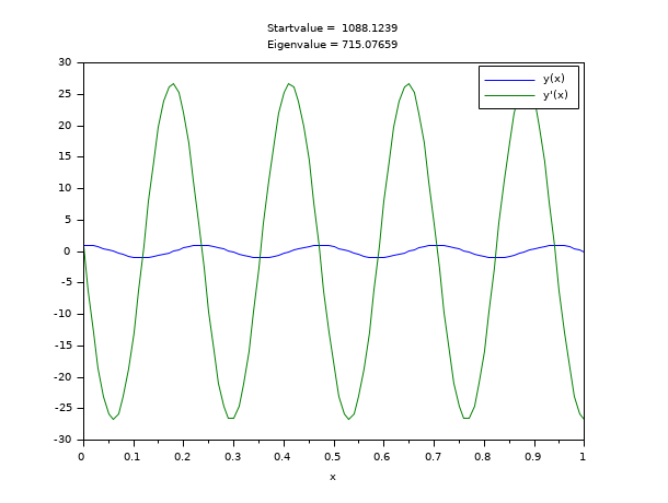
An eigenvalue problem:
// y''(x)=-la*y(x)
// BV: y(0)=y'(0); y(1)=0
// Eigenfunctions and eigenvalues are y(x,n)=sin(s(n)*(1-x)), la(n)=s(n)^2,
// where s(n) are the zeros of f(s,n)=s+atan(s)-(n+1)*pi, n=0,1,2,...
// To get a third boundary condition, we choose y(0)=1
// (With y(x) also c*y(x) is a solution for each constant c.)
// We solve the following ode system:
// y''=-la*y
// la'=0
// BV: y(0)=y'(0), y(0)=1; y(1)=0
// z=[y(x) ; y'(x) ; la]

function rhs=fsub(x, z)
  rhs=[-z(3)*z(1);0]
endfunction

function g=gsub(i, z)
  g=[z(1)-z(2) z(1)-1 z(1)]
  g=g(i)
endfunction

// The following start function is good for the first 8 eigenfunctions.
function [z, lhs]=ystart(x, z, la0)
  z=[1;0;la0]
  lhs=[0;0]
endfunction

a=0;b=1;
m=[2;1];
n=2;
zeta=[a a b];
N=101;
x=linspace(a,b,N)';

// We have s(n)-(n+1/2)*pi -> 0 for n to infinity.
la0=evstr(x_dialog('n-th eigenvalue: n= ?','10'));
la0=(%pi/2+la0*%pi)^2;

z=bvodeS(x,m,n,a,b,fsub,gsub,zeta,ystart=list(ystart,la0));
// The same call without any display
z=bvodeS(x,m,n,a,b,fsub,gsub,zeta,ystart=list(ystart,la0),iprint=1);
// The same with a lot of display
z=bvodeS(x,m,n,a,b,fsub,gsub,zeta,ystart=list(ystart,la0),iprint=-1);

clf()
plot(x,[z(1,:)' z(2,:)'])
xtitle(['Startvalue =  '+string(la0);'Eigenvalue = '+string(z(3,1))],'x',' ')
legend(['y(x)';'y''(x)']);
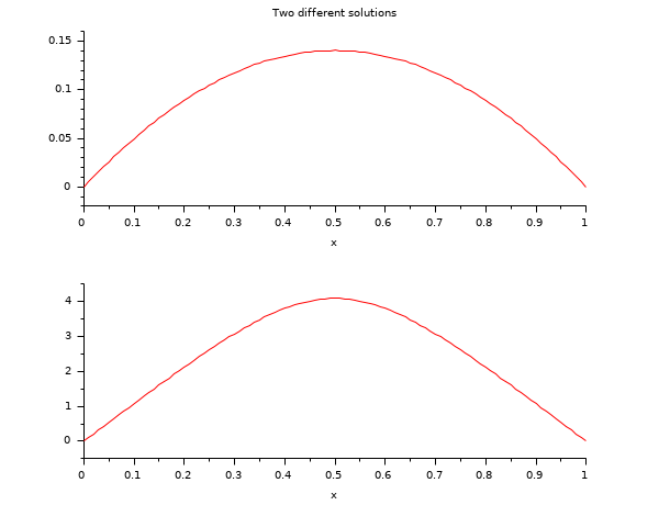
A boundary value problem with more than one solution.
// DE: y''(x)=-exp(y(x))
// BV: y(0)=0; y(1)=0
// This boundary value problem has more than one solution.
// It is demonstrated how to find two of them with the help of
// some preinformation of the solutions y(x) to build the function ystart.
// z=[y(x);y'(x)]

a=0;
b=1;
m=2;
n=1;
zeta=[a b];
N=101;
tol=1e-8*[1 1];
x=linspace(a,b,N);

function rhs=fsub(x, z)
  rhs=-exp(z(1));
endfunction

function g=gsub(i, z)
  g=[z(1) z(1)]
  g=g(i)
endfunction

function [z, lhs]=ystart(x, z, M)
  //z=[4*x*(1-x)*M ; 4*(1-2*x)*M]
  z=[M;0]
  //lhs=[-exp(4*x*(1-x)*M)]
  lhs=0
endfunction

for M=[1 4]
   if M==1
      z=bvodeS(x,m,n,a,b,fsub,gsub,zeta,ystart=list(ystart,M),tol=tol);
   else
      z1=bvodeS(x,m,n,a,b,fsub,gsub,zeta,ystart=list(ystart,M),tol=tol);
   end
end

// Integrating the ode yield e.g. the two solutions yex and yex1.

function y=f(c)
  y=c.*(1-tanh(sqrt(c)/4).^2)-2;
endfunction
c=fsolve(2,f);

function y=yex(x, c)
  y=log(c/2*(1-tanh(sqrt(c)*(1/4-x/2)).^2))
endfunction

function y=f1(c1), y=2*c1^2+tanh(1/4/c1)^2-1;endfunction
c1=fsolve(0.1,f1);

function y=yex1(x, c1)
  y=log((1-tanh((2*x-1)/4/c1).^2)/2/c1/c1)
endfunction

disp(norm(z(1,:)-yex(x)),'norm(yex(x)-z(1,:))= ')
disp(norm(z1(1,:)-yex1(x)),'norm(yex1(x)-z1(1,:))= ')
clf();
subplot(2,1,1)
plot2d(x,z(1,:),style=[5])
xtitle('Two different solutions','x',' ')
subplot(2,1,2)
plot2d(x,z1(1,:),style=[5])
xtitle(' ','x',' ')
A multi-point boundary value problem.
// DE y'''(x)=1
// z=[y(x);y'(x);y''(x)]
// BV: y(-1)=2 y(1)=2
// Side condition: y(0)=1

a=-1;b=1;c=0;
// The side condition point c must be included in the array fixpnt.
n=1;
m=[3];

function rhs=fsub(x, z)
  rhs=1
endfunction

function g=gsub(i, z)
  g=[z(1)-2 z(1)-1 z(1)-2]
  g=g(i)
endfunction

N=10;
zeta=[a c b];
x=linspace(a,b,N);

z=bvodeS(x,m,n,a,b,fsub,gsub,zeta,fixpnt=c);

function y=yex(x)
y=x.^3/6+x.^2-x./6+1
endfunction

disp(norm(yex(x)-z(1,:)),'norm(yex(x)-z(1,:))= ')
Quantum Neumann equation, with 2 "eigenvalues" (c_1 and c2). Continuation being used.
// Quantum Neumann equation, with 2 "eigenvalues" c_1 and c_2
// (c_1=v-c_2-c_3, v is a parameter, used in continuation)
//
// diff(f,x,2) + (1/2)*(1/x + 1/(x-1) + 1/(x-y))*diff(f,x)
//      - (c_1/x + c_2/(x-1) + c_3/(x-y))* f(x) = 0
// diff(c_2,x)=0,  diff(c_3,x) = 0
//
// and 4 "boundary" conditions: diff(f,x)(a_k)=2*c_k*f(a_k) for
// k=1,2,3, a_k=(0, 1 , y)  and normalization f(1) = 1
//
// The z-vector is z_1=f, z_2=diff(f,x), z_3=c_2 and z_4=c_3
// The guess is chosen to have one node in [0,1],  f(x)=2*x-1
// such that f(1)=1, c_2 and c_3 are chosen to cancel poles in
// the differential equation at 1.0 and y, z_3=1, z_4=1/(2*y-1)
// Ref: http://arxiv.org/pdf/hep-th/0407005

y= 1.9d0;
eigens=zeros(3,40); // To store the results

// General setup for bvode

// Number of differential equations
ncomp = 3;

// Orders of equations
m = [2, 1, 1];

// Non-linear problem
ipar(1) = 1;

// Number of collocation points
ipar(2) = 3;

// Initial uniform mesh of 4 subintervals
ipar(3) = 4;
ipar(8) = 0;

// Size of fspace, ispace, see colnew.f to choose size
ipar(5) =  30000;
ipar(6) =  2000;

// Medium output
ipar(7) = 0;

// Initial approx is provided
ipar(9) = 1;

// fixpnt is an array containing all fixed points in the mesh, in
// particular "boundary" points, except aleft and aright, ipar[11] its
// size, here only one interior "boundary point"
ipar(11) = 1;
fixpnt = [1.0d0];

// Tolerances on all components z_1, z_2, z_3, z_4
ipar(4) = 4;

// Tolerance check on f and diff(f,x) and on c_2 and c_3
ltol = [1, 2, 3, 4];
tol = [1d-5, 1d-5, 1d-5, 1d-5];

// Define the differential equations

function [f]=fsub(x, z)
    f = [ -.5*(1/x+1/(x-1)+1/(x-y))*z(2) +...
     z(1) * ((v-z(3)-z(4))/x + z(3)/(x-1) + z(4)/(x-y)),...
    0,0];
endfunction
function [df]=dfsub(x, z)
    df = [(v-z(3)-z(4))/x + z(3)/(x-1) + z(4)/(x-y),...
    -.5*(1/x+1/(x-1)+1/(x-y)),z(1)/(x*(x-1)),z(1)*y/(x*(x-y));...
    0,0,0,0;0,0,0,0];
endfunction

// Boundary conditions

function [g]=gsub(i, z)
    select i
    case 1, g = z(2) - 2*z(1)*(v-z(3)-z(4))
    case 2, g = z(2) - 2*z(1)*z(3)
    case 3, g = z(1)-1.
    case 4, g = z(2) - 2*z(1)*z(4)
    end
endfunction
function [dg]=dgsub(i, z)
        select i
        case 1, dg = [-2*(v-z(3)-z(4)),1.,2*z(1),2*z(1)]
        case 2, dg = [-2*z(3),1.,-2*z(1),0]
        case 3, dg = [1,0,0,0]
        case 4, dg = [-2*z(4),1.,0,-2*z(1)]
        end
endfunction

// Start computation

// Locations of side conditions, sorted
zeta = [0.0d0, 1.0d0, 1.0d0, y];
// Interval ends
aleft = 0.0d0;
aright = y;

// Array of 40 values of v explored by continuation, and array of 202
// points where to evaluate function f.
valv = [linspace(0,.9,10) logspace(0,2,30)];
res = [linspace(0,.99,100) linspace(1,y,101)];

// eigenstates are characterized by number of nodes in [0,1] and in
// [1,y], here guess selects one node (zero) in [0,1] with linear
// f(x)=2*x-1 and constant c_2, c_3, so dmval=0. Notice that the z-vector
// has mstar = 4 components, while dmval has ncomp = 3 components.

function [z, dmval]=guess(x)
     z=[2*x-1, 2., 1., 1/(2*y-1)]
     dmval=[0,0,0]
endfunction

// First execution has ipar(9)=1 and uses the guess
// Subsequent executions have ipar(9)=3 and use continuation. This is
// run in tight closed loop to not disturb the stack

for i=1:40
v=valv(i);
sol=bvode(res,ncomp,m,aleft,aright,zeta,ipar,ltol,tol,fixpnt,...
 fsub,dfsub,gsub,dgsub,guess);
eigens(:,i)=[v;sol(3,101);sol(4,101)];  // c_2 and c_3 are constant!
ipar(9)=3;
end

// To see the evolution of the eigenvalues with v, disp(eigens)
// Note they evolve smoothly.
// To see the solution f for v=40, disp(sol(1,:)). Note that it vanishes
// exactly once in [0,1] at x close to 0.98, and becomes very small
// when x -> 0 and very large when x -> y.
// This is markedly different from the case  at small v.
// The continuation procedure allows to explore these exponential behaviours
// without skipping to other eigenstates.
See also
Used Functions
This function is based on the Fortran routine
colnew developed by
U. Ascher, Department of Computer Science, University of British Columbia, Vancouver, B.C. V6T 1W5, Canada
G. Bader, institut f. Angewandte mathematik university of Heidelberg; im Neuenheimer feld 294d-6900 Heidelberg 1
Bibliography
U. Ascher, J. Christiansen and R.D. Russell, collocation software for boundary-value ODEs, acm trans. math software 7 (1981), 209-222. this paper contains EXAMPLES where use of the code is demonstrated.
G. Bader and U. Ascher, a new basis implementation for a mixed order boundary value ode solver, siam j. scient. stat. comput. (1987).
U. Ascher, J. Christiansen and R.D. Russell, a collocation solver for mixed order systems of boundary value problems, math. comp. 33 (1979), 659-679.
U. Ascher, J. Christiansen and R.D. russell, colsys - a collocation code for boundary value problems, lecture notes comp.sc. 76, springer verlag, b. children et. al. (eds.) (1979), 164-185.
C. Deboor and R. Weiss, solveblok: a package for solving almost block diagonal linear systems, acm trans. math. software 6 (1980), 80-87.
| Report an issue | ||
| << Differential calculus, Integration | Differential calculus, Integration | dae >> |