Please note that the recommended version of Scilab is 2026.1.0. This page might be outdated.
See the recommended documentation of this function
eval_cshep2d
bidimensional cubic shepard interpolation evaluation
Syntax
zp                                            = eval_cshep2d(xp, yp, tl_coef)
[zp, dzpdx, dzpdy]                            = eval_cshep2d(xp, yp, tl_coef)
[zp, dzpdx, dzpdy, d2zpdxx, d2zpdyy, d2zpdxy] = eval_cshep2d(xp, yp, tl_coef)
Arguments
- xp, yp
two real vectors (or matrices) of the same size
- tl_coef
a tlist scilab structure (of type cshep2d) defining a cubic Shepard interpolation function (named
Sin the following)- zp
vector (or matrix) of the same size than
xpandyp, evaluation of the interpolantSat these points- dzpdx,dzpdy
vectors (or matrices) of the same size than
xpandyp, evaluation of the first derivatives ofSat these points- d2zpdxx,d2zpdxy,d2zpdyy
vectors (or matrices) of the same size than
xpandyp, evaluation of the second derivatives ofSat these points
Description
This is the evaluation routine for cubic Shepard interpolation function computed with cshep2d, that is :

Remark
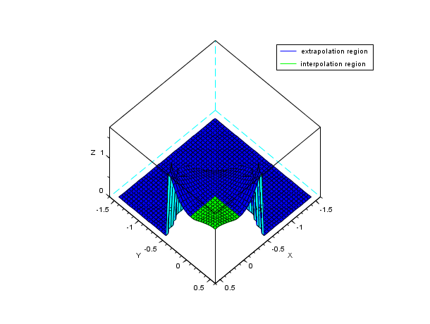
The interpolant S is C2 (twice continuously differentiable) but is also extended by zero for (x,y) far enough the interpolation points. This leads to a discontinuity in a region far outside the interpolation points, and so, is not cumbersome in practice (in a general manner, evaluation outside interpolation points (i.e. extrapolation) leads to very inaccurate results).
Examples
// see example section of cshep2d

// this example shows the behavior far from the interpolation points ...
deff("z=f(x,y)","z = 1+ 50*(x.*(1-x).*y.*(1-y)).^2")
x = linspace(0,1,10);
[X,Y] = ndgrid(x,x);
X = X(:); Y = Y(:); Z = f(X,Y);
S = cshep2d([X Y Z]);
// evaluation inside and outside the square [0,1]x[0,1]
m = 40;
xx = linspace(-1.5,0.5,m);
[xp,yp] = ndgrid(xx,xx);
zp = eval_cshep2d(xp,yp,S);
// compute facet (to draw one color for extrapolation region
// and another one for the interpolation region)
[xf,yf,zf] = genfac3d(xx,xx,zp);
colors = 2*ones(1,size(zf,2));
// indices corresponding to facet in the interpolation region
ind=find( mean(xf,"r")>0 & mean(xf,"r")<1 & mean(yf,"r")>0 & mean(yf,"r")<1 );
colors(ind)=3;
clf();
plot3d(xf,yf,list(zf,colors), flag=[2 6 4])
legends(["extrapolation region","interpolation region"],[2 3],1)
show_window()
See also
- cshep2d — bidimensional cubic shepard (scattered) interpolation
History
| Version | Description |
| 5.4.0 | previously, imaginary part of input arguments were implicitly ignored. |
| Report an issue | ||
| << cshep2d | Interpolation | interp >> |