lsq_splin

Arguments

xd, yd

vectors of the same size, data to be fitted by a cubic spline

wd

(optional) a vector of same format than xd and yd, weights of the least square fit.

x

a strictly increasing (row or column) vector, breakpoints of the cubic spline

y, d

vectors of same format than x, the triplet (x,y,d) defines the approximated cubic spline.

Description

This function computes an approximated cubic spline s for the data xd, yd, wd (in the following m is supposed to be the length of these vectors) and from a choice of the spline breakpoints x (for instance if you want n breakpoints uniformly chosen you may use x=linspace(min(xd),max(xd),n))). If S is the space of all cubic splines functions with breakpoints x1 < x2 < ... < xn then the resulting spline s is such that:

for all fin S, i.e. realizes the minimum of the sum of the squared errors over all functions of S.

The spline s is completely defined by the triplet (x,y,d) (y and d are the vectors of the spline ordinates and first derivatives at the xi 's : yi=s(xi) and di=s'(xi)) and its evaluation at some points must be done by the interp function.

Remarks

When wd is not given, all the points have the same weight 1.

A point (xd(k),yd(k)) is considered in the fit if xd(k) in [x1,xn] and wd(k) > 0. In particular you can put a null (or even negative) weight to all data points you want to ignore in the fitting. When the total number of points taken into account in the fit procedure is (strictly) less than 4 an error is issued.

The vector xd do not need to be in increasing order.

Depending on the number and on the positions of the xd(k) 's and on the choice of the x(i) 's there may be several solutions but only one is selected. When this occurs a warning message is displayed in the Scilab command window. This function is intended to be used when m is much larger than n and in this case no such problem may occurred.

Examples

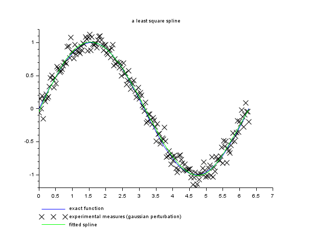
// this is an artificial example where the data xd and yd
// are build from a perturbed sin function
a = 0; b = 2*%pi;
sigma = 0.1;  // standard deviation of the gaussian noise
m = 200;       // number of experimental points
xd = linspace(a,b,m)';
yd = sin(xd) + grand(xd,"nor",0,sigma);

n = 6; // number of breakpoints
x = linspace(a,b,n)';

// compute the spline
[y, d] = lsq_splin(xd, yd, x);  // use equal weights

// plotting
ye = sin(xd);
ys = interp(xd, x, y, d);
clf()
plot2d(xd,[ye yd ys],style=[2 -2 3], ...
       leg="exact function@experimental measures (gaussian perturbation)@fitted spline")
xtitle("a least square spline")
show_window()

See also

• interp — cubic spline evaluation function
• splin — cubic spline interpolation