- Scilab Help
- Graphics
- 2d_plot
- LineSpec
- Matplot
- Matplot1
- Matplot properties
- Sfgrayplot
- Sgrayplot
- champ
- champ1
- champ properties
- comet
- contour2d
- contour2di
- contour2dm
- contourf
- errbar
- fchamp
- fec
- fec properties
- fgrayplot
- fplot2d
- grayplot
- grayplot properties
- graypolarplot
- histplot
- paramfplot2d
- plot
- plot2d
- plot2d2
- plot2d3
- plot2d4
- polarplot
- scatter
Please note that the recommended version of Scilab is 2026.1.0. This page might be outdated.
See the recommended documentation of this function
Sfgrayplot
smooth 2D plot of a surface defined by a function using colors
Syntax
Sfgrayplot(x, y, f, <opt_args>)
Sfgrayplot(x, y, f [,strf, rect, nax, zminmax, colminmax, mesh, colout])
Arguments
- x, y
real row vectors of size
n1andn2.- f
a scilab function (
z=f(x,y)).- <opt_args>
this represents a sequence of statements
key1=value1, key2=value2, ...wherekey1,key2, ...can be one of the following:strf,rect,nax,zminmax,colminmax,mesh,colout(see plot2d for the 3 first and fec for the 4 last).- strf, rect, nax
see plot2d.
- zminmax, colminmax, mesh, colout
see fec.
Description
Sfgrayplot is the same as fgrayplot but the
plot is smoothed. The function fec is used for smoothing. The
surface is plotted assuming that it is linear on a set of triangles built
from the grid (here with n1=5, n2=3):
_____________
| /| /| /| /|
|/_|/_|/_|/_|
| /| /| /| /|
|/_|/_|/_|/_|
The function colorbar may be used to see the color scale (but you must know (or compute) the min and max values).
Instead of Sfgrayplot, you can use Sgrayplot and this may be
a little faster.
Enter the command Sfgrayplot() to see a demo.
Examples
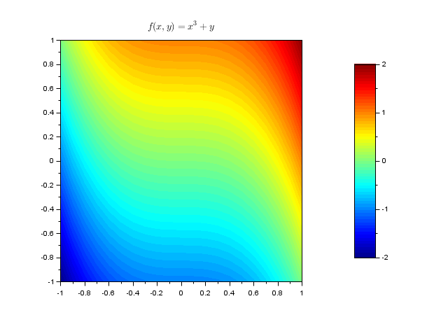
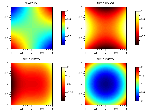
// example #1: plot 4 surfaces
function z=surf1(x, y), z=x*y, endfunction
function z=surf2(x, y), z=x^2-y^2, endfunction
function z=surf3(x, y), z=x^3+y^2, endfunction
function z=surf4(x, y), z=x^2+y^2, endfunction
clf()
set(gcf(),"color_map",[jetcolormap(64);hotcolormap(64)])
x = linspace(-1,1,60);
y = linspace(-1,1,60);
drawlater();
subplot(2,2,1)
  colorbar(-1,1,[1,64])
  Sfgrayplot(x,y,surf1,strf="041",colminmax=[1,64])
  xtitle("f(x,y) = x*y")
subplot(2,2,2)
  colorbar(-1,1,[65,128])
  Sfgrayplot(x,y,surf2,strf="041",colminmax=[65,128])
  xtitle("f(x,y) = x^2-y^2")
subplot(2,2,3)
  colorbar(-1,2,[65,128])
  Sfgrayplot(x,y,surf3,strf="041",colminmax=[65,128])
  xtitle("f(x,y) = x^3+y^2")
subplot(2,2,4)
  colorbar(0,2,[1,64])
  Sfgrayplot(x,y,surf4,strf="041",colminmax=[1,64])
  xtitle("f(x,y) = x^2+y^2")
drawnow();
show_window()
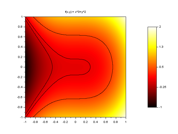
// example #2: plot surf3 and add some contour lines
function z=surf3(x, y), z=x^3+y^2, endfunction
clf()
x = linspace(-1,1,60);
y = linspace(-1,1,60);
set(gcf(),"color_map",hotcolormap(128))
drawlater();
colorbar(-1,2)
Sfgrayplot(x,y,surf3,strf="041")
contour2d(x,y,surf3,[-0.1, 0.025, 0.4],style=[1 1 1],strf="000")
xtitle("f(x,y) = x^3+y^2")
drawnow();
show_window()
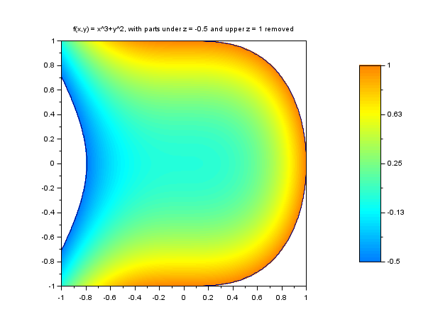
// example #3: plot surf3 and use zminmax and colout optional arguments
//             to restrict the plot for -0.5<= z <= 1
function z=surf3(x, y), z=x^3+y^2, endfunction
clf()
x = linspace(-1,1,60);
y = linspace(-1,1,60);
set(gcf(),"color_map",jetcolormap(128))
drawlater();
zminmax = [-0.5 1]; colors=[32 96];
colorbar(zminmax(1),zminmax(2),colors)
Sfgrayplot(x, y, surf3, strf="041", zminmax=zminmax, colout=[0 0], colminmax=colors)
contour2d(x,y,surf3,[-0.5, 1],style=[1 1 1],strf="000")
xtitle("f(x,y) = x^3+y^2, with parts under z = -0.5 and upper z = 1 removed")
drawnow();
show_window()
See also
| Report an issue | ||
| << Matplot properties | 2d_plot | Sgrayplot >> |