Please note that the recommended version of Scilab is 2026.1.0. This page might be outdated.
See the recommended documentation of this function
rpem
再帰的予測誤差最小推定
呼び出し手順
[w1,[v]]=rpem(w0,u0,y0,[lambda,[k,[c]]])
引数
- w0
list(theta,p,l,phi,psi)ただし:- theta
[a,b,c] はi
3*n次の実数ベクトルです- a,b,c
a=[a(1),...,a(n)], b=[b(1),...,b(n)], c=[c(1),...,c(n)]
- p
(3*n x 3*n) 実数行列.
- phi,psi,l
3*n次の実数ベクトル
最初のコールで適用可能な値を以下に示します:
- u0
入力の実数ベクトル (任意の大きさ). (
u0($)は rpemで使用されません)- y0
出力のベクトル (
u0と同じ次元). (y0(1)はrpemでは使用されません).時間領域が
(t0,t0+k-1)の場合,u0ベクトルは入力u(t0),u(t0+1),..,u(t0+k-1)およびy0は出力y(t0),y(t0+1),..,y(t0+k-1)を有します.
オプションの引数
- lambda
オプションの引数 (忘却定数) 収束した時に1に近くなるように選択:
lambda=[lambda0,alfa,beta]は下式に基づき更新されます :lambda(t)=alfa*lambda(t-1)+beta
ただし,
lambda(0)=lambda0です.- k
収束した際に1に近くなるように選択される縮小係数.
k=[k0,mu,nu]は下式に基づき更新されます:k(t)=mu*k(t-1)+nu
ただし,
k(0)=k0です.- c
大きな引数(
c=1000がデフォルト値です).
出力:
- w1
w0の更新.- v
u0, y0における二乗予測誤差の合計(オプション).特に
w1(1)はthetaの新しい推定値です. 新しい標本u1, y1が利用できる時, 以下のように更新が行われます:[w2,[v]]=rpem(w1,u1,y1,[lambda,[k,[c]]]). 任意の大きな級数を扱うことができます.
説明
ARMAXモデルの引数の再帰的推定. Ljung-Soderstromの再帰的予測誤差法を使用します. 考慮されるモデルを以下に示します:
y(t)+a(1)*y(t-1)+...+a(n)*y(t-n)=
b(1)*u(t-1)+...+b(n)*u(t-n)+e(t)+c(1)*e(t-1)+...+c(n)*e(t-n)
このコマンドの効果は,未知の引数theta=[a,b,c]の
推定値を更新することです.
ただし,a=[a(1),...,a(n)], b=[b(1),...,b(n)], c=[c(1),...,c(n)]です.
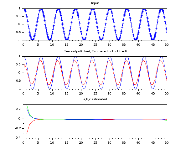
例
nbPoints = 50; // Number of points computed

// Real parameters a,b,c: here, y=u
a=cat(2,1,zeros(1,nbPoints - 1));
b=cat(2,1,zeros(1,nbPoints - 1));
c=zeros(1,nbPoints);

// Generate input signal
t=linspace(0,50,600);
w=%pi/3;
u=cos(w*t);

// Generate output signal
Arma=armac(a,b,c,1,1,0);
y=arsimul(Arma,u);

f1=figure("figure_name","figure1","backgroundColor",[1 1 1]);
subplot(3,1,1);
plot(t, u, "b+");
xtitle("Input");
subplot(3,1,2);
plot(t, y);

// Arguments of rpem
phi=zeros(1,nbPoints*3);
psi=zeros(1,nbPoints*3);
l=zeros(1,nbPoints*3);
p=1*eye(nbPoints*3,nbPoints*3);
theta=[0*a 0*b 0*c];
w0=list(theta,p,l,phi,psi);
[w0, v]=rpem(w0,u,y);

// Get estimated parameters:
a_est=w0(1)(1);
b_est=w0(1)(nbPoints + 1);
c_est=w0(1)(2 * nbPoints + 1);
for i=2:nbPoints
    a_est=cat(2,a_est,w0(1)(i));
    b_est=cat(2,b_est,w0(1)(i+nbPoints));
    c_est=cat(2,c_est,w0(1)(i+2*nbPoints));
end

// Generate and plot output estimated
Arma_est=armac(a_est,b_est,c_est,1,1,0);
y_est=arsimul(Arma_est,u);
plot(t, y_est,"color","red");
xtitle("Real output(blue), Estimated output (red)");

// Plot estimated parameters
subplot(3,1,3);
xtitle("a,b,c estimated");
plot(a_est(1,:),"color","red");
plot(b_est(1,:),"color","green");
plot(c_est(1,:),"color","blue");
| Report an issue | ||
| << phc | Identification | Miscellaneous >> |