Please note that the recommended version of Scilab is 2026.1.0. This page might be outdated.
See the recommended documentation of this function
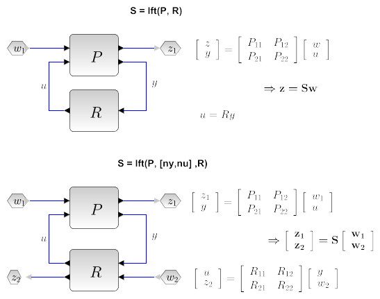
lft
linear fractional transformation
Syntax
S=lft(P,R)
[S,s]=lft(P,p,R [,r])
Arguments
- P
linear system (in state space or transfer function representation) or a simple gain, the ``augmented'' plant, implicitly partitioned into four blocks (two input ports and two output ports).
- p
1x2 row vector, the dimensions of the
P_22block (see below).- R
llinear system (in state space or transfer function representation) or a simple gain, implicitly partitioned into four blocks (two input ports and two output ports).
- r
1x2 row vector, dimension of the
R_22block . This argument should not be used. It is retained for compatibility with previous versions.- S
linear system, the linear fractional transform.
- s
1x2 row vector, dimension of the
S_22block (see below).
Description
Linear fractional transform between two standard plants in state space form or in transfer form:
- Syntax
S=lft(P,R) Computes the linear fractional transform between the systems
Pand a controllerR. The systemScorresponds to the transfer
if
nyandnuare respectively the number of inputs and outputs ofR, one must havesize(P)>=[ny nu]. The system returned is formally equivalent toUsingi1 = 1:($-ny);j1=1:($-nu); i2 = ($-ny+1):$;j1=($-nu+1):$; S = P(i1,j1) + P(i1,j2) * R * (eye() - P(i2,j2) * R) \P(i2,j1)
lftinstead of the code above avoids numerical problems and non minimal realization.- Syntax
[S,s]=lft(P,p,R) with
p= [ny,nu]Forms the generalized (2 ports) lft ofPandR.Sis the two-port interconnected plant, which correspond to the transfer:
sis the dimension of the22block ofS.
P and R can be PSSDs i.e. may admit a
polynomial D matrix.
Examples
See also
| Report an issue | ||
| << feedback | Boucles de contrôle | Découplage des perturbations >> |