svplot

Arguments

sl

syslin list (continuous, discrete or sampled system)

w

real vector (optional parameter)

Description

computes for the system sl=(A,B,C,D) the singular values of its transfer function matrix:

G(jw) = C(jw*I-A)B^-1+D
or
G(exp(jw)) = C(exp(jw)*I-A)B^-1+D
or
G(exp(jwT)) = C(exp(jw*T)*I-A)B^-1+D

evaluated over the frequency range specified by w. (T is the sampling period, T=sl('dt') for sampled systems).

sl is a syslin list representing the system [A,B,C,D] in state-space form. sl can be continuous or discrete time or sampled system.

The i-th column of the output matrix SVM contains the singular values of G for the i-th frequency value w(i).

SVM = svplot(sl)

is equivalent to

SVM = svplot(sl,logspace(-3,3))  (continuous)

SVM = svplot(sl,logspace(-3,%pi)) (discrete)

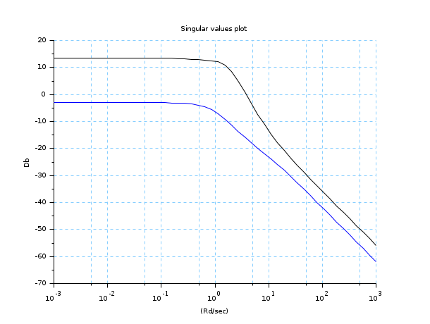
Examples

x=logspace(-3,3);
y=svplot(ssrand(2,2,4),x);
clf();plot2d1("oln",x',20*log(y')/log(10));
xgrid(12)
xtitle("Singular values plot","(Rd/sec)", "Db");