Please note that the recommended version of Scilab is 2026.1.0. This page might be outdated.
See the recommended documentation of this function
optim_sa
A Simulated Annealing optimization method
Calling Sequence
x_best = optim_sa(x0,f,ItExt,ItInt,T0,Log,temp_law,param_temp_law,neigh_func,param_neigh_func)
[x_best,f_best] = optim_sa(..)
[x_best,f_best,mean_list] = optim_sa(..)
[x_best,f_best,mean_list,var_list] = optim_sa(..)
[x_best,f_best,mean_list,var_list,f_history] = optim_sa(..)
[x_best,f_best,mean_list,var_list,f_history,temp_list] = optim_sa(..)
[x_best,f_best,mean_list,var_list,f_history,temp_list,x_history] = optim_sa(..)
[x_best,f_best,mean_list,var_list,f_history,temp_list,x_history,iter] = optim_sa(..)
Arguments
- x0
the initial solution
- f
the objective function to be optimized (the prototype if f(x))
- ItExt
the number of temperature decrease
- ItInt
the number of iterations during one temperature stage
- T0
the initial temperature (see compute_initial_temp to compute easily this temperature)
- Log
if %T, some information will be displayed during the run of the simulated annealing
- temp_law
the temperature decrease law (see temp_law_default for an example of such a function)
- param_temp_law
a structure (of any kind - it depends on the temperature law used) which is transmitted as a parameter to temp_law
- neigh_func
a function which computes a neighbor of a given point (see neigh_func_default for an example of such a function)
- param_neigh_func
a structure (of any kind like vector, list, it depends on the neighborhood function used) which is transmitted as a parameter to neigh_func
- x_best
the best solution found so far
- f_best
the objective function value corresponding to x_best
- mean_list
the mean of the objective function value for each temperature stage. A vector of float (optional)
- var_list
the variance of the objective function values for each temperature stage. A vector of float (optional)
- f_history
the computed objective function values for each iteration. Each input of the list corresponds to a temperature stage. Each input of the list is a vector of float which gathers all the objective function values computed during the corresponding temperature stage - (optional)
- temp_list
the list of temperature computed for each temperature stage. A vector of float (optional)
- x_history
the parameter values computed for each iteration. Each input of the list corresponds to a temperature stage. Each input of the list is a vector of input variables which corresponds to all the variables computed during the corresponding temperature stage - (optional - can slow down a lot the execution of optim_sa)
- iter
a double, the actual number of external iterations in the algorithm (optional).
Description
A Simulated Annealing optimization method.
Simulated annealing (SA) is a generic probabilistic meta-algorithm for the global optimization problem, namely locating a good approximation to the global optimum of a given function in a large search space. It is often used when the search space is discrete (e.g., all tours that visit a given set of cities).
The current solver can find the solution of an optimization problem without constraints or with bound constraints. The bound constraints can be customized with the neighbour function. This algorithm does not use the derivatives of the objective function.
The solver is made of Scilab macros, which enables a high-level programming model for
this optimization solver. The SA macros are based on the parameters
Scilab module for the management of the (many) optional parameters.
To use the SA algorithm, one should perform the following steps :
- configure the parameters with calls to
init_paramandadd_paramespecially the neighbor function, the acceptance function, the temperature law, - compute an initial temperature with a call to
compute_initial_temp, - find an optimum by using the
optim_sasolver.
The algorithm is based on an iterative update of two points :
- the current point is updated by taking into account the neighbour and the acceptance functions,
- the best point is the point which achieved the minimum of the objective function over the iterations.
The acceptance of the new point depends on the output values produced
by the rand function. This implies that two consecutive
calls to the optim_sa will not produce the same result.
In order to always get exactly the same results, please initialize the random number
generator with a valid seed.
See the Demonstrations, in the "Optimization" section and "Simulated Annealing" subsection for more examples.
The objective function
The objective function is expected to have the following header.
function y=f(x)
In the case where the objective function needs additional parameters, the objective function can be defined as a list, where the first argument is the cost function, and the second argument is the additional parameter. See below for an example.
Examples
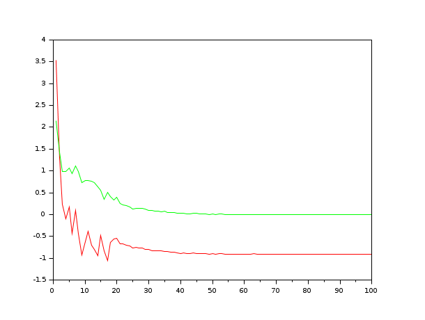
In the following example, we search the minimum of the Rastriging function. This function has many local minimas, but only one single global minimum located at x = (0,0), where the function value is f(x) = -2. We use the simulated annealing algorithm with default settings and the default neighbour function neigh_func_default.
function y=rastrigin(x)
  y = x(1)^2+x(2)^2-cos(12*x(1))-cos(18*x(2));
endfunction

x0          = [2 2];
Proba_start = 0.7;
It_Pre      = 100;
It_extern   = 100;
It_intern   = 1000;
x_test = neigh_func_default(x0);

T0 = compute_initial_temp(x0, rastrigin, Proba_start, It_Pre);

Log = %T;
[x_opt, f_opt, sa_mean_list, sa_var_list] = optim_sa(x0, rastrigin, It_extern, It_intern, T0, Log);

mprintf("optimal solution:\n"); disp(x_opt);
mprintf("value of the objective function = %f\n", f_opt);

t = 1:length(sa_mean_list);
plot(t,sa_mean_list,"r",t,sa_var_list,"g");
Configuring a neighbour function
In the following example, we customize the
neighbourhood function. In order to pass this function to the
optim_sa function, we setup a parameter where the
"neigh_func" key is associated with our particular neighbour function.
The neighbour function can be customized at will, provided that the
header of the function is the same. The particular implementation shown
below is the same, in spirit, as the neigh_func_default
function.
function f=quad(x)
  p = [4 3];
  f = (x(1) - p(1))^2 + (x(2) - p(2))^2
endfunction

// We produce a neighbor by adding some noise to each component of a given vector
function x_neigh=myneigh_func(x_current, T, param)
  nxrow = size(x_current,"r")
  nxcol = size(x_current,"c")
  sa_min_delta = -0.1*ones(nxrow,nxcol);
  sa_max_delta = 0.1*ones(nxrow,nxcol);
  x_neigh = x_current + (sa_max_delta - sa_min_delta).*rand(nxrow,nxcol) + sa_min_delta;
endfunction

x0          = [2 2];
Proba_start = 0.7;
It_Pre      = 100;
It_extern   = 50;
It_intern   = 100;

saparams = init_param();
saparams = add_param(saparams,"neigh_func", myneigh_func);
// or: saparams = add_param(saparams,"neigh_func", neigh_func_default);
// or: saparams = add_param(saparams,"neigh_func", neigh_func_csa);
// or: saparams = add_param(saparams,"neigh_func", neigh_func_fsa);
// or: saparams = add_param(saparams,"neigh_func", neigh_func_vfsa);

T0 = compute_initial_temp(x0, quad, Proba_start, It_Pre, saparams);
Log = %f;
// This should produce x_opt = [4 3]
[x_opt, f_opt] = optim_sa(x0, quad, It_extern, It_intern, T0, Log, saparams)
Passing extra parameters
In the following example, we use an objective function which requires
an extra parameter p. This parameter is the second
input argument of the quadp function. In order to
pass this parameter to the objective function, we define the objective
function as list(quadp,p). In this case,
the solver makes so that the calling sequence includes a second argument.
function f=quadp(x, p)
f = (x(1) - p(1))^2 + (x(2) - p(2))^2
endfunction

x0 = [-1 -1];
p = [4 3];
Proba_start = 0.7;
It_Pre      = 100;
T0 = compute_initial_temp(x0, list(quadp,p) , Proba_start, It_Pre);
[x_opt, f_opt] = optim_sa(x0, list(quadp,p) , 10, 1000, T0, %f)
Configuring an output function
In the following example, we define an output function, which also
provide a stopping rule. We define the function outfun
which takes as input arguments the data of the algorithm at the current
iteration and returns the boolean stop. This function
prints a message into the console to inform the user about the
current state of the algorithm. It also computes the boolean stop,
depending on the value of the function.
The stop variable becomes true when the function value is near zero. In order to let optim_sa
know about our output function, we configure the "output_func"
key to our outfun function and call the solver.
Notice that the number of external iterations is %inf, so
that the external loop never stops.
This allows to check that the output function really allows to
stop the algorithm.
function f=quad(x)
  p = [4 3];
  f = (x(1) - p(1))^2 + (x(2) - p(2))^2
endfunction

function stop=outfunc(itExt, x_best, f_best, T, saparams)
  [mythreshold,err] = get_param(saparams,"mythreshold",0);
  mprintf ( "Iter = #%d, \t x_best=[%f %f], \t f_best = %e, \t T = %e\n", itExt , x_best(1),x_best(2) , f_best , T )
  stop = ( abs(f_best) < mythreshold )
endfunction

x0 = [-1 -1];
saparams = init_param();
saparams = add_param(saparams,"output_func", outfunc );
saparams = add_param(saparams,"mythreshold", 1.e-2 );

rand("seed",0);

T0 = compute_initial_temp(x0, quad , 0.7, 100, saparams);
[x_best, f_best, mean_list, var_list, temp_list, f_history, x_history , It ] = optim_sa(x0, quad , %inf, 100, T0, %f, saparams);
The previous script produces the following output. Notice that the actual
output of the algorithm depends on the state of the random number generator rand:
if we had not initialize the seed of the uniform random number generator,
we would have produced a different result.
Iter = #1,      x_best=[-1.000000 -1.000000],      f_best = 4.100000e+001,      T = 1.453537e+000
Iter = #2,      x_best=[-0.408041 -0.318262],      f_best = 3.044169e+001,      T = 1.308183e+000
Iter = #3,      x_best=[-0.231406 -0.481078],      f_best = 3.002270e+001,      T = 1.177365e+000
Iter = #4,      x_best=[0.661827 0.083743],      f_best = 1.964796e+001,      T = 1.059628e+000
Iter = #5,      x_best=[0.931415 0.820681],      f_best = 1.416565e+001,      T = 9.536654e-001
Iter = #6,      x_best=[1.849796 1.222178],      f_best = 7.784028e+000,      T = 8.582988e-001
Iter = #7,      x_best=[2.539775 1.414591],      f_best = 4.645780e+000,      T = 7.724690e-001
Iter = #8,      x_best=[3.206047 2.394497],      f_best = 9.969957e-001,      T = 6.952221e-001
Iter = #9,      x_best=[3.164998 2.633170],      f_best = 8.317924e-001,      T = 6.256999e-001
Iter = #10,      x_best=[3.164998 2.633170],      f_best = 8.317924e-001,      T = 5.631299e-001
Iter = #11,      x_best=[3.164998 2.633170],      f_best = 8.317924e-001,      T = 5.068169e-001
Iter = #12,      x_best=[3.961464 2.903763],      f_best = 1.074654e-002,      T = 4.561352e-001
Iter = #13,      x_best=[3.961464 2.903763],      f_best = 1.074654e-002,      T = 4.105217e-001
Iter = #14,      x_best=[3.961464 2.903763],      f_best = 1.074654e-002,      T = 3.694695e-001
Iter = #15,      x_best=[3.931929 3.003181],      f_best = 4.643767e-003,      T = 3.325226e-001
See Also
- compute_initial_temp — A SA function which allows to compute the initial temperature of the simulated annealing
- neigh_func_default — A SA function which computes a neighbor of a given point
- temp_law_default — A SA function which computed the temperature of the next temperature stage
Bibliography
"Simulated annealing : theory and applications", P.J.M. Laarhoven and E.H.L. Aarts, Mathematics and its applications, Dordrecht : D. Reidel, 1988
"Theoretical and computational aspects of simulated annealing", P.J.M. van Laarhoven, Amsterdam, Netherlands : Centrum voor Wiskunde en Informatica, 1988
"Genetic algorithms and simulated annealing", Lawrence Davis, London : Pitman Los Altos, Calif. Morgan Kaufmann Publishers, 1987
| Report an issue | ||
| << Algorithms | Algorithms | Utilities >> |