Please note that the recommended version of Scilab is 2026.1.0. This page might be outdated.
See the recommended documentation of this function
bode
Bode plot
Calling Sequence
bode(sl, [fmin, fmax] [,step] [,comments] )
bode(sl, [fmin, fmax] [,step] [,comments] [,"rad"] )
bode(sl, frq [,comments] )
bode(sl, frq [,comments] [,"rad"] )
bode(frq, db, phi [,comments] )
bode(frq, repf [,comments] [,"rad"] )
Arguments
- sl
syslinlist (SISO or SIMO linear system) in continuous or discrete time.- fmin,fmax
real (frequency bounds (in Hz))
- step
real (logarithmic step.)
- comments
vector of character strings (captions).
- frq
row vector or matrix (frequencies (in Hz) ) (one row for each SISO subsystem).
- db
row vector or matrix ( magnitudes (in Db)). (one row for each SISO subsystem).
- phi
row vector or matrix ( phases (in degree)) (one row for each SISO subsystem).
- repf
row vector or matrix of complex numbers (complex frequency response).
- "rad"
converts the frequency from Hz into rad/s (multiplies by 2π),
Description
Bode plot, i.e magnitude and phase of the frequency response of
sl.
sl can be a continuous-time or discrete-time SIMO
system (see syslin). In case of multi-output the
outputs are plotted with different symbols.
The frequencies are given by the bounds fmin,fmax
(in Hz) or by a row-vector (or a matrix for multi-output)
frq.
step is the ( logarithmic ) discretization step.
(see calfrq for the choice of default value).
comments is a vector of character strings
(captions).
db,phi are the matrices of modulus (in Db) and
phases (in degrees). (One row for each response).
repf matrix of complex numbers. One row for each
response.
Default values for fmin and
fmax are 1.d-3,
1.d+3 if sl is continuous-time or
1.d-3, 0.5/sl.dt (nyquist frequency)
if sl is discrete-time. Automatic discretization of
frequencies is made by calfrq.
The datatips tool may be used to display data along the phase and modulus curves.
Examples
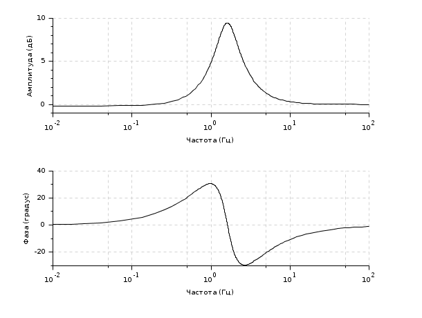
s = poly(0, 's');
h = syslin('c', (s^2+2*0.9*10*s+100)/(s^2+2*0.3*10.1*s+102.01));

clf(); bode(h, 0.01, 100);
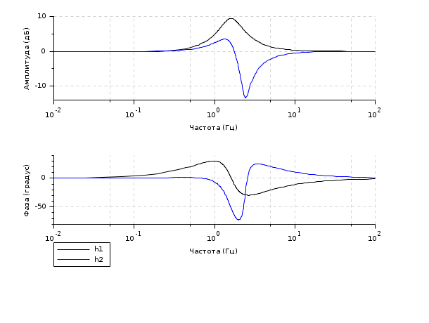
s = poly(0, 's');
h1 = syslin('c', (s^2+2*0.9*10*s+100)/(s^2+2*0.3*10.1*s+102.01));
num = 22801+4406.18*s+382.37*s^2+21.02*s^3+s^4;
den = 22952.25+4117.77*s+490.63*s^2+33.06*s^3+s^4;
h2 = syslin('c', num/den);

clf(); bode([h1; h2], 0.01, 100, ['h1'; 'h2']);
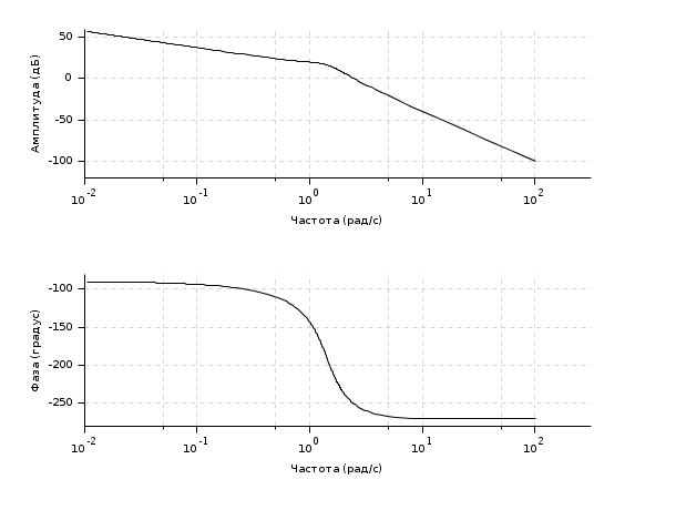
s = %s;
G = (10*(s+3))/(s*(s+2)*(s^2+s+2)); // A rational matrix
sys = syslin('c', G); // A continuous-time linear system in transfer matrix representation.
f_min = .0001; f_max = 16; // Frequencies in Hz

clf(); bode(sys, f_min, f_max, "rad"); // Converts Hz to rad/s
See Also
- bode_asymp — Bode plot asymptote
- black — Black-Nichols diagram of a linear dynamical system
- nyquist — nyquist plot
- gainplot — magnitude plot
- repfreq — frequency response
- g_margin — gain margin and associated crossover frequency
- p_margin — phase margin and associated crossover frequency
- calfrq — frequency response discretization
- phasemag — phase and magnitude computation
- datatips — Tool for placing and editing tips along the plotted curves.
| Report an issue | ||
| << black | Plot and display | bode_asymp >> |