Please note that the recommended version of Scilab is 2026.1.0. This page might be outdated.
See the recommended documentation of this function
rpem
Recursive Prediction-Error Minimization estimation
Calling Sequence
[w1,[v]]=rpem(w0,u0,y0,[lambda,[k,[c]]])
Arguments
- w0
list(theta,p,l,phi,psi)where:- theta
[a,b,c] is a real vector of order
3*n- a,b,c
a=[a(1),...,a(n)], b=[b(1),...,b(n)], c=[c(1),...,c(n)]
- p
(3*n x 3*n) real matrix.
- phi,psi,l
real vector of dimension
3*n
Applicable values for the first call:
- u0
real vector of inputs (arbitrary size). (
u0($)is not used by rpem)- y0
vector of outputs (same dimension as
u0). (y0(1)is not used by rpem).If the time domain is
(t0,t0+k-1)theu0vector contains the inputsu(t0),u(t0+1),..,u(t0+k-1)andy0the outputsy(t0),y(t0+1),..,y(t0+k-1)
Optional arguments
- lambda
optional argument (forgetting constant) choosed close to 1 as convergence occur:
lambda=[lambda0,alfa,beta]evolves according to :lambda(t)=alfa*lambda(t-1)+beta
with
lambda(0)=lambda0- k
contraction factor to be chosen close to 1 as convergence occurs.
k=[k0,mu,nu]evolves according to:k(t)=mu*k(t-1)+nu
with
k(0)=k0.- c
Large argument.(
c=1000is the default value).
Outputs:
- w1
Update for
w0.- v
sum of squared prediction errors on
u0, y0.(optional).In particular
w1(1)is the new estimate oftheta. If a new sampleu1, y1is available the update is obtained by:[w2,[v]]=rpem(w1,u1,y1,[lambda,[k,[c]]]). Arbitrary large series can thus be treated.
Description
Recursive estimation of arguments in an ARMAX model. Uses Ljung-Soderstrom recursive prediction error method. Model considered is the following:
y(t)+a(1)*y(t-1)+...+a(n)*y(t-n)=
b(1)*u(t-1)+...+b(n)*u(t-n)+e(t)+c(1)*e(t-1)+...+c(n)*e(t-n)
The effect of this command is to update the estimation of
unknown argument theta=[a,b,c] with
a=[a(1),...,a(n)], b=[b(1),...,b(n)], c=[c(1),...,c(n)].
Example
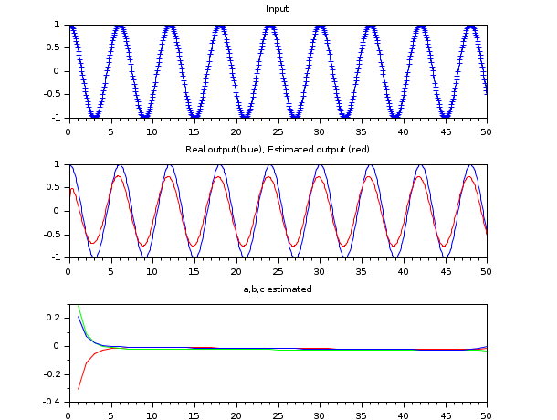
nbPoints = 50; // Number of points computed

// Real parameters a,b,c: here, y=u
a=cat(2,1,zeros(1,nbPoints - 1));
b=cat(2,1,zeros(1,nbPoints - 1));
c=zeros(1,nbPoints);

// Generate input signal
t=linspace(0,50,600);
w=%pi/3;
u=cos(w*t);

// Generate output signal
Arma=armac(a,b,c,1,1,0);
y=arsimul(Arma,u);

f1=figure("figure_name","figure1","backgroundColor",[1 1 1]);
subplot(3,1,1);
plot(t, u, "b+");
xtitle("Input");
subplot(3,1,2);
plot(t, y);

// Arguments of rpem
phi=zeros(1,nbPoints*3);
psi=zeros(1,nbPoints*3);
l=zeros(1,nbPoints*3);
p=1*eye(nbPoints*3,nbPoints*3);
theta=[0*a 0*b 0*c];
w0=list(theta,p,l,phi,psi);
[w0, v]=rpem(w0,u,y);

// Get estimated parameters:
a_est=w0(1)(1);
b_est=w0(1)(nbPoints + 1);
c_est=w0(1)(2 * nbPoints + 1);
for i=2:nbPoints
    a_est=cat(2,a_est,w0(1)(i));
    b_est=cat(2,b_est,w0(1)(i+nbPoints));
    c_est=cat(2,c_est,w0(1)(i+2*nbPoints));
end

// Generate and plot output estimated
Arma_est=armac(a_est,b_est,c_est,1,1,0);
y_est=arsimul(Arma_est,u);
plot(t, y_est,"color","red");
xtitle("Real output(blue), Estimated output (red)");

// Plot estimated parameters
subplot(3,1,3);
xtitle("a,b,c estimated");
plot(a_est(1,:),"color","red");
plot(b_est(1,:),"color","green");
plot(c_est(1,:),"color","blue");
| Report an issue | ||
| << phc | identification | miscellaneous >> |