Please note that the recommended version of Scilab is 2026.1.0. This page might be outdated.
See the recommended documentation of this function
interp
cubic spline evaluation function
Calling Sequence
[ yp [,yp1 [,yp2 [,yp3]]]] = interp(xp, x, y, d [, out_mode])
Arguments
- x,y
real vectors of same size
n: Coordinates of data points on which the interpolation and the related cubic spline (calleds(X)in the following) or sub-spline function is based and built.- d
real vector of size(x): The derivative s'(x). Most often, s'(x) will be priorly estimated through the function splin(x, y,..)
- out_mode
(optional) string defining
s(X)forXoutside .
Possible values: "by_zero" | "by_nan" | "C0" | "natural" | "linear" | "periodic"
.
Possible values: "by_zero" | "by_nan" | "C0" | "natural" | "linear" | "periodic"- xp
real vector or matrix: abscissae at which
Yis unknown and must be estimated withs(xp)- yp
vector or matrix of size(xp):
yp(i) = s(xp(i))oryp(i,j) = s(xp(i,j))- yp1, yp2, yp3
vectors (or matrices) of size(x): elementwise evaluation of the derivatives
s'(xp),s''(xp)ands'''(xp).
Description
The cubic spline function s(X) interpolating the (x,y) set of given points is a continuous and derivable piece-wise function defined over  . It consists of a set of cubic polynomials, each one
  being defined on
  and connected in values and slopes to both its neighbours. Thus, we can state that for each
  , such that
 . Then, interp() evaluates
 s(X) (and s'(X), s''(X), s'''(X) if needed) at xp(i), such that


The out_mode parameter set the evaluation rule
for extrapolation, i.e. for xp(i) outside  :
:
- "by_zero"
an extrapolation by zero is done
- "by_nan"
extrapolation by Nan (%nan)
- "C0"
the extrapolation is defined as follows :


- "natural"
the extrapolation is defined as follows (
 being the polynomial defining
s(X)on )
)

- "linear"
the extrapolation is defined as follows :


- "periodic"
s(X)is extended by periodicity:
Examples
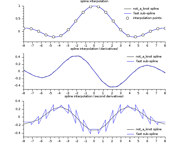
// see the examples of splin and lsq_splin

// an example showing C2 and C1 continuity of spline and subspline
a = -8; b = 8;
x = linspace(a,b,20)';
y = sinc(x);
dk = splin(x,y);  // not_a_knot
df = splin(x,y, "fast");
xx = linspace(a,b,800)';
[yyk, yy1k, yy2k] = interp(xx, x, y, dk);
[yyf, yy1f, yy2f] = interp(xx, x, y, df);
clf()
subplot(3,1,1)
plot2d(xx, [yyk yyf])
plot2d(x, y, style=-9)
legends(["not_a_knot spline","fast sub-spline","interpolation points"],...
        [1 2 -9], "ur",%f)
xtitle("spline interpolation")
subplot(3,1,2)
plot2d(xx, [yy1k yy1f])
legends(["not_a_knot spline","fast sub-spline"], [1 2], "ur",%f)
xtitle("spline interpolation (derivatives)")
subplot(3,1,3)
plot2d(xx, [yy2k yy2f])
legends(["not_a_knot spline","fast sub-spline"], [1 2], "lr",%f)
xtitle("spline interpolation (second derivatives)")
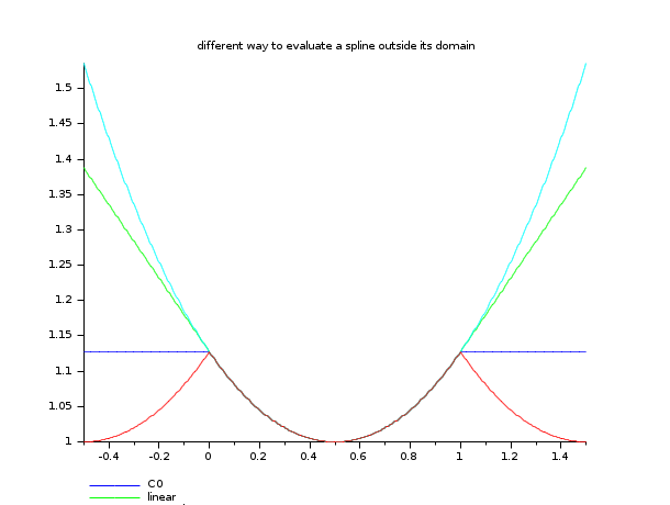
// here is an example showing the different extrapolation possibilities
x = linspace(0,1,11)';
y = cosh(x-0.5);
d = splin(x,y);
xx = linspace(-0.5,1.5,401)';
yy0 = interp(xx,x,y,d,"C0");
yy1 = interp(xx,x,y,d,"linear");
yy2 = interp(xx,x,y,d,"natural");
yy3 = interp(xx,x,y,d,"periodic");
clf()
plot2d(xx,[yy0 yy1 yy2 yy3],style=2:5,frameflag=2,leg="C0@linear@natural@periodic")
xtitle(" different way to evaluate a spline outside its domain")
History
| Version | Description |
| 5.4.0 | previously, imaginary part of input arguments were implicitly ignored. |
| Report an issue | ||
| << eval_cshep2d | Interpolation | interp1 >> |