PID

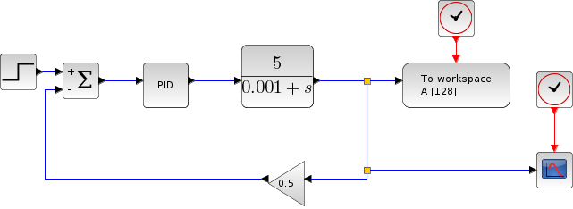
Block Screenshot

Contents

• PID regulator

• • Palette

  • Description

  • Dialog box

  • Default properties

  • Interfacing function

  • Compiled Super Block content

  • Examples

Palette

• Continuous time systems palette

Description

This block implements a PID (Proportional-Integral-Differential) controller. It calculates an "error" value Ue as the difference between a measured process variable Upr and a desired setpoint Ur.

The purpose is to make the process variable Up follow the setpoint value Ur. The PID controller is widely used in feedback control of industrial processes.

The PID controller calculation (algorithm) involves three separate parameters; the Proportional Kp, the Integral Ki and Derivative Kd values. These terms describe three basic mathematical functions applied to the error signal Ue. Kp determines the reaction to the current error, Ki determines the reaction based on the sum of recent errors and Kd determines the reaction to the rate at which the error has been changing.

The weighted sum of these three actions is used to adjust the process via a control element such as the position of a control valve or the power supply of a heating element. The basic structure of conventional feedback control systems is shown below:

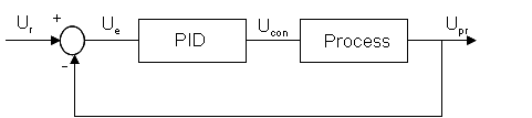
PID law is a linear combinaison of an input variable Up(t), its time integral Ui(t) and its first derivative Ud(t). The control law Ucon(t) has the form:

Dialog box

• Proportional

  The value of the gain that multiply the error.

  Properties : Type 'vec' of size -1.

• Integral

  The value of the integral time of the error.(1/Integral)

  Properties : Type 'vec' of size -1.

• Derivation

  The value of the derivative time of the error.

  Properties : Type 'vec' of size -1.

Default properties

• always active: no

• direct-feedthrough: no

• zero-crossing: no

• mode: no

• regular inputs:

  - port 1 : size [-1,-2] / type 1

• regular outputs:

  - port 1 : size [-1,-2] / type 1

• number/sizes of activation inputs: 0

• number/sizes of activation outputs: 0

• continuous-time state: no

• discrete-time state: no

• object discrete-time state: no

• name of computational function: csuper

Interfacing function

• SCI/modules/scicos_blocks/macros/Linear/PID.sci

Compiled Super Block content

Example 1

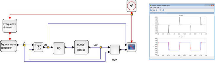
This example illustrates the usage of PID regulator. It enables you to fit the output signal Upr(t) to the required signal Ur(t) easily.

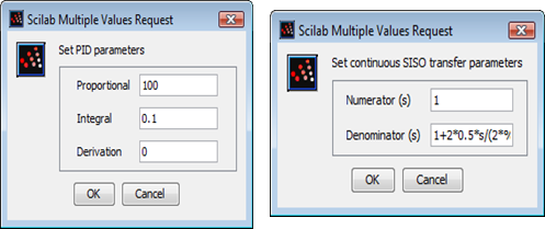
In this example the control system is a second-order unity-gain low-pass filter with damping ratio ξ=0.5 and cutoff frequency fc= 100 Hz. Its transfer function H(s) is:

To model this filter we use Continuous transfer function block (CLR) from Continuous time systems Palette.

The PID parameters Kp, Ki and Kd are set to 100, 0.1 and 0.

The scope displays the waveforms of system error Ue (black), reference signal Ur (blue) and process signal Upr(red). It shows how initially the process signal Upr(t) does not follow the reference signal Ur(t).

Example 2

Example 3