dsearch
distribute, locate and count elements of a matrix or hypermatrix in given categories
Syntax
[i_bin [,counts [,outside]]] = dsearch(X, bins )
[i_bin [,counts [,outside]]] = dsearch(X, bins , pm )
Arguments
- X
matrix or hypermatrix of reals, encoded integers, or texts: The entries to categorize. Complex numbers and polynomials are not supported.
- bins
row or column vector defining categories, of same type as
X(for encoded integers inX,binsmay be decimals).- Discrete case (pm="d"):
binsare distinct values to whichXentries must be identified. IfXis numeric (reals or encoded integers),binsmust be sorted in strictly increasing order. - Continuous case (default, pm="c"):
binsare bounds of contiguous intervals:I1 = [bins(1), bins(2)],I2 = (bins(2), bins(3)],...,In = (bins(n), bins(n+1)]. Note that entries fromXjust equal to bins(1) are included inI1. The values inbinsmust be in strictly increasing order: bins(1) < bins(2) < ... < bins(n). For text processing, the case-sensitive lexicographic order is considered.
- Discrete case (pm="d"):
- pm
"c" (continuous, default) or "d" (discrete): processing mode. In continuous mode,
binsdefines the bounds of contiguous intervals considered as categories. In discrete mode,binsprovides the values to which entries fromXmust be identified.- i_bin
matrix or hypermatrix with same sizes than
X:i_bin(k)is the index of the category to whichX(k)belongs. IfX(k)belongs to none of the categories,i_bin(k) = 0- counts
- number of X entries in respective bins.
Continuous case (pm="c"): counts(i) elements of
Xbelong to the intervalIkas defined above (see thebinsparameter). Elements ofXjust equal to bins(1) are included in counts(1).countshas the size ofbins- 1Discrete case (pm="d"):
counts(i)elements ofXare equal tobins(i) - outside
Total number of X entries belonging to none of the
bins.
Description
For each X(i) entry, dsearch locates the value bins(j) or the interval (bins(j), bins(j+1)] defined by bins and containing or equal to X(i). Then it returns i_bin(i) = j or 0 whether no bin equals or contains it. (the first interval includes bins(1)). The population of each bin is returned through counts. The total number of unbinned entries is returned in outside (therefore outside = sum(bool2s(i_bin==0))).
dsearch(..) can be overloaded.
The default pm="c" option can be used to compute the empirical histogram of a function given a dataset.
Examples
// DISCRETE values of TEXT
// -----------------------
i = grand(4,6,"uin",0,7)+97;
T = matrix(strsplit(ascii(i),1:length(i)-1), size(i));
T(T=="f") = "#";
T(T=="a") = "AA";
T
bins = [ strsplit(ascii(97+(7:-1:0)),1:7)' "AA"]
[i_bin, counts, outside] = dsearch(T, bins, "d")

// BINNING TEXTS in LEXICOGRAPHIC INTERVALS
// ----------------------------------------
// generating a random matrix of text
nL = 3; nC = 5; L  = 3;
s = ascii(grand(1,nL*nC*L,"uin",0,25)+97);
T = matrix(strsplit(s, L:L:nL*nC*L-1), nL, nC);
// generating random bins bounds
L  = 2; nC = 6;
s = ascii(grand(1,nC*L,"uin",0,25)+97);
bins = unique(matrix(strsplit(s, L:L:nC*L-1), 1, nC))
T
[i_bin, counts, outside] = dsearch(T, bins)
In the following example, we consider 3 intervals I1 = [5,11],
I2 = (11,15] and I3 = (15,20].
We are looking for the location of the entries of X = [11 13 1 7 5 2 9]
in these intervals.
[i_bin, counts, outside] = dsearch([11 13 1 7 5 2 9], [5 11 15 20])
Displayed output:
-->[i_bin, counts, outside] = dsearch([11 13 1 7 5 2 9], [5 11 15 20])
 outside  =
    2.
 counts  =
    4.    1.    0.
 i_bin  =
    1.    2.    0.    1.    1.    0.    1.
Indeed,
X(1)=11 is in the interval I1, hence i_bin(1)=1.
X(2)=13 is in the interval I2, hence i_bin(2)=2.
X(3)=1 belongs to none of defined intervals, hence i_bin(3)=0.
X(4)=7 is in the interval I1, hence i_bin(4)=1.
...
There are four X entries (5, 7, 9 and 11) in I1, hence counts(1)=4.
There is only one X entry (13) in I2, hence counts(2)=1.
There is no X entry in I3, hence counts(3)=0.
There are two X entries (i.e. 1, 2) which belong to none of defined intervals, hence outside=2.
// Numbers in DISCRETE categories (having specific values)
// ------------------------------
[i_bin, counts, outside] = dsearch([11 13 1 7 5 2 9], [5 11 15 20],"d" )
displays
-->[i_bin, counts, outside] = dsearch([11 13 1 7 5 2 9], [5 11 15 20], "d" )
 outside  =
    5.
 counts  =
    1.    1.    0.    0.
 i_bin  =
    2.    0.    0.    0.    1.    0.    0.
Indeed,
X(1)=11 is in the set
binsat position #2, hence i_bin(1)=2.X(2)=13 is not in the set
bins, hence i_bin(2)=0....
X(7)=9 is not in the set
bins, hence i_bin(7)=0.There is only one entry X (i.e. 5) equal to 5, hence counts(1)=1.
There are no entries matching
bins(4), hence counts(4)=0.There are five X entries (i.e. 13, 1, 7, 2, 9) which are not in the set
bins, hence outside=5.
Numbers in bins must be in increasing order, whatever is the processing mode (continuous or discrete).
If this is not the case, an error is generated:
-->dsearch([11 13 1 7 5 2 9], [2 1])
!--error 999
dsearch   : the array s (arg 2) is not well ordered
-->dsearch([11 13 1 7 5 2 9], [2 1],"d")
!--error 999
dsearch   : the array s (arg 2) is not well ordered
Advanced Examples
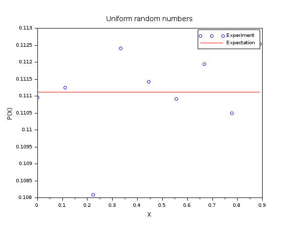
In the following example, we compare the empirical histogram of uniform random numbers in [0,1) with the uniform distribution function. To perform this comparison, we use the default search algorithm based on intervals (pm="c"). We generate X as a collection of m=50 000 uniform random numbers in the range [0,1). We consider the n=10 values equally equally spaced values in the [0,1] range and consider the associated intervals. Then we count the number of entries in X which fall in the intervals: this is the empirical histogram of the uniform distribution function. The expectation for counts/m is equal to 1/(n-1).
m = 50000 ;
n = 10;
X = grand(m, 1, "def");
bins = linspace(0, 1, n)';
[i_bin, counts] = dsearch(X, bins);
e = 1/(n-1)*ones(1, n-1);
scf() ;
plot(bins(1:n-1), counts/m, "bo");
plot(bins(1:n-1), e', "r-");
legend(["Experiment", "Expectation"]);
xtitle("Uniform random numbers", "X", "P(X)");
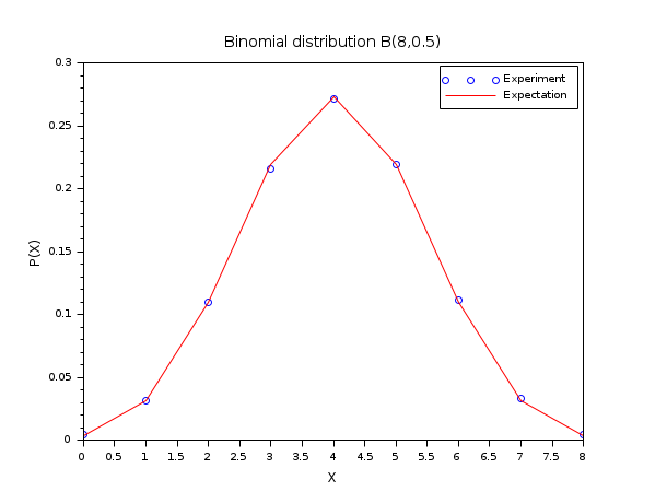
In the following example, we compare the histogram of binomially distributed random numbers with the binomial probability distribution function B(N,p), with N=8 and p=0.5. To perform this comparison, we use the discrete search algorithm based on a set (pm="d").
N = 8 ;
p = 0.5;
m = 50000;
X = grand(m,1,"bin",N,p);
bins = (0:N)';
[i_bin, counts] = dsearch(X, bins, "d");
Pexp = counts/m;
Pexa = binomial(p,N);
scf() ;
plot(bins, Pexp, "bo");
plot(bins, Pexa', "r-");
xtitle("Binomial distribution B(8,0.5)","X","P(X)");
legend(["Experiment","Expectation"]);
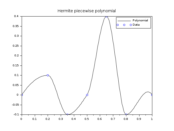
In the following example, we use piecewise Hermite polynomials to interpolate a dataset.
// define Hermite base functions
function y=Ll(t, k, x)
  // Lagrange left on Ik
  y=(t-x(k+1))./(x(k)-x(k+1))
endfunction
function y=Lr(t, k, x)
  // Lagrange right on Ik
  y=(t-x(k))./(x(k+1)-x(k))
endfunction
function y=Hl(t, k, x)
  y=(1-2*(t-x(k))./(x(k)-x(k+1))).*Ll(t,k,x).^2
endfunction
function y=Hr(t, k, x)
  y=(1-2*(t-x(k+1))./(x(k+1)-x(k))).*Lr(t,k,x).^2
endfunction
function y=Kl(t, k, x)
  y=(t-x(k)).*Ll(t,k,x).^2
endfunction
function y=Kr(t, k, x)
  y=(t-x(k+1)).*Lr(t,k,x).^2
endfunction

x = [0 ; 0.2 ; 0.35 ; 0.5 ; 0.65 ; 0.8 ;  1];
y = [0 ; 0.1 ;-0.1  ; 0   ; 0.4  ;-0.1 ;  0];
d = [1 ; 0   ; 0    ; 1   ; 0    ; 0   ; -1];
X = linspace(0, 1, 200)';
i_bin = dsearch(X, x);

// plot the curve
Y = y(i_bin).*Hl(X,i_bin) + y(i_bin+1).*Hr(X,i_bin) + d(i_bin).*Kl(X,i_bin) + d(i_bin+1).*Kr(X,i_bin);
scf();
plot(X,Y,"k-");
plot(x,y,"bo")
xtitle("Hermite piecewise polynomial");
legend(["Polynomial","Data"]);
// NOTE : it can be verified by adding these ones :
// YY = interp(X,x,y,d); plot2d(X,YY,3,"000")
See also
History
| Version | Description |
| 5.5.0 | Extension to hypermatrices, encoded integers, and text. |
| Report an issue | ||
| << Search and sort | Search and sort | find >> |