FROMWSB
Data from Scilab workspace to Xcos
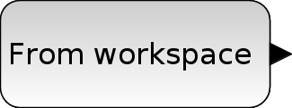
Block Screenshot

Contents
Description
That block is used to get data defined in the Scilab workspace and use them in Xcos. Data should have "time" and "values" fields.
Parameters

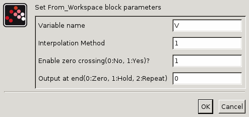
Variable name. The variable must be a structure defined in Scilab, with two fields:
.timeis a column vector of real numbers, of size (Nx1) ;.valuesis a matrix with N rows, whose type can be be , , , , , , , and .Interpolation method: Variables read by Xcos are data values read at discrete instants given by the time field. This option causes the block to interpolate at time steps for which no corresponding workspace data exists. There are four interpolation methods available.
0: "Zero order method". This method generates a piecewise constant signal. i.e., for
ti ≤ t < ti+1,y(t) = yi. This method is available for all data types.1: "Linear method". This method generates a piecewise linear signal, i.e., for
ti ≤ t < ti+1,y(t) = yi + (yi+1-yi)/ (ti+1-ti)For data types other than double and complex, the linear interpolation can be used, but the final output will be computed by casting interpolation result into the original data type.2:"NATURAL method". This cubic spline is computed by using the following conditions (considering
npointsx_1, ..., x_n):
This method is only available for Real and complex data types.
3:"NOT_A_KNOT method". The cubic spline is computed by using the following conditions (considering
npointsx_1, ..., x_n) :
This method is only available for Real and Complex data types.
Enable zero crossing(0:No, 1:Yes)?: Enables zero crossing detection. When and interpolation methods are chosen, the output signal will be discontinuous at data time instants. These possible discontinuities may cause problem for the numerical solver. In order to perform a reliable numerical integration, the zero crossing option is used. If output of the block affects data used by the numerical solver, at discontinuous points, a discrete event is generated and the numerical solver is cold restarted. The discrete event is also generated at the
t_1andt_nfor other interpolating methods.Output at end(0:Zero, 1:Hold, 2:Repeat): This option is for selecting method for generating output after the last time point for which data is available from the workspace.
0("Zero"): The output is set to zero.
1("Hold"): The output is hold.
2("Repeat"): The output is repeated from workspace.
Default properties
always active: no
direct-feedthrough: no
zero-crossing: no
mode: no
regular outputs:
- port 1 : size [-1,1] / type 1
number/sizes of activation inputs: 0
number/sizes of activation outputs: 0
continuous-time state: no
discrete-time state: no
object discrete-time state: no
name of computational function: csuper
Example
// Create the variable to load from
V.time = (1:1000)'; //the values must be on a column vector
V.values = cos(2* %pi * V.time / 20);

Interfacing function
SCI/modules/scicos_blocks/macros/Sources/FROMWSB.sci
See also
- TOWS_c — Data to Scilab workspace
| Report an issue | ||
| << CURV_f | Sources_pal | GENSIN_f >> |