phaseplot
frequency phase plot
Syntax
phaseplot(sl)
phaseplot(sl, fmin, fmax)
phaseplot(sl, fmin, fmax, step)
phaseplot(frq, db, phi)
phaseplot(frq, repf)
phaseplot(.., comments)
Arguments
- sl
A siso or simo linear dynamical system, in state space, transfer function or zpk representations, in continuous or discrete time.
- fmin
real scalar: the minimum frequency (in Hz) to be represented.
- fmax
real scalar: the maximum frequency (in Hz) to be represented.
- step
real scalar: the frequency discretization step (logarithmic scale)). If it is not specified the algorithm uses adaptative frequency steps.
- comments
a character string vector: the legend label to be associated with each curve. Optional value is the empty array.
- frq
a row vector or an n x m array: The frequency discretization in Hz.
- db
an n x m array: the magnitudes corresponding to
frq. This argument is not used, it only appears to makephaseplothave the same syntax asgainplotandbode.- phi
an n x m array: the phases in degree corresponding to
frq. Thephaseplotfunction plots the curvesphi(i,:)versusfrq(i,:)- repf
an n x m complex array. The
phaseplotfunction plots the curvesphase(repf(i,:))versusfrq(i,:)
Description
This function draws the phase of the frequency response of a system. The system can be given under different representations:
phaseplot(sl,...)caseslcan be a continuous-time or discrete-time SIMO system given by its state space, rational transfer function (see syslin) or zpk representation. In case of multi-output the outputs are plotted with different colors.In this case the frequencies can be given by:
the lower and upper bounds in Hz
fmin,fmaxand an optional frequency stepstep. The default values forfminandfmaxare1.e-3,1.e3ifslis continuous-time or1.e-3,0.5/sl.dt(nyquist frequency) ifslis discrete-time. If thestepargument is omitted the function use an adaptative frequency step (see calfrq).a row vector or a 2D array
frqwhich gives the frequency values in Hz. 2D array can be used for multi-output systems if one wants to have different frequency discretization for each input/output couple.
phaseplot(frq,...)caseThis case allows to draw frequency phase plots for previously computed frequency responses. The frequency response can be given either by it's complex representation
repfor by it's magnitude phase representationdb,phi.frqandrepfmust be row vectors or n x m arrays (each row represent an input/output couple).
The datatips tool may be used to display data along the phase curves.
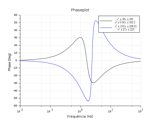
Examples
s=poly(0,'s')
h1=syslin('c',(s^2+2*0.9*10*s+100)/(s^2+2*0.3*10.1*s+102.01))
h2=syslin('c',(s^2+2*0.1*15.1*s+228.01)/(s^2+2*0.9*15*s+225))
clf();phaseplot([h1;h2],0.01,100,..
                   ["$\frac{s^2+18 s+100}{s^2+6.06 s+102.1}$";
                    "$\frac{s^2+3.02 s+228.01}{s^2+27 s+225}$"])
title('Phaseplot')
See also
History
| Versão | Descrição |
| 5.4.0 | Function phaseplot introduced. |
| 6.0 | handling zpk representation. |
| Report an issue | ||
| << phasemag | Frequency Domain | repfreq >> |