armax
armax identification
Syntax
[arc, la, lb, sig, resid] = armax(r, s, y, u)
[arc, la, lb, sig, resid] = armax(r, s, y, u, b0f, prf)
Arguments
- y
output process y(ny,n); ( ny: dimension of y , n : sample size)
- u
input process u(nu,n); ( nu: dimension of u , n : sample size)
- r and s
auto-regression orders r >=0 et s >=-1
- b0f
optional parameter. Its default value is 0 and it means that the coefficient b0 must be identified. if bof=1 the b0 is supposed to be zero and is not identified
- prf
optional parameter for display control. If prf =1, the default value, a display of the identified Arma is given.
- arc
a Scilab arma object (see armac)
- la
is the list(a,a+eta,a-eta) ( la = a in dimension 1) ; where eta is the estimated standard deviation. , a=[Id,a1,a2,...,ar] where each ai is a matrix of size (ny,ny)
- lb
is the list(b,b+etb,b-etb) (lb =b in dimension 1) ; where etb is the estimated standard deviation. b=[b0,.....,b_s] where each bi is a matrix of size (nu,nu)
- sig
is the estimated standard deviation of the noise and resid=[ sig*e(t0),....] (
Description
armax is used to identify the coefficients of a n-dimensional ARX process
A(z^-1)y= B(z^-1)u + sig*e(t)
where e(t) is a n-dimensional white noise with variance I. sig an nxn matrix and A(z) and B(z):
A(z) = 1+a1*z+...+a_r*z^r; ( r=0 => A(z)=1)
B(z) = b0+b1*z+...+b_s z^s ( s=-1 => B(z)=0)
for the method see Eykhoff in trends and progress in system identification, page 96.
with
z(t)=[y(t-1),..,y(t-r),u(t),...,u(t-s)]
and
coef= [-a1,..,-ar,b0,...,b_s]
we can write
y(t)= coef* z(t) + sig*e(t) and the algorithm minimises
sum_{t=1}^N ( [y(t)- coef'z(t)]^2)
where t0=max(max(r,s)+1,1))).
Examples
//-Ex1- Arma model : y(t) = 0.2*u(t-1)+0.01*e(t-1)
ny=1,nu=1,sig=0.01;
Arma=armac(1,[0,0.2],[0,1],ny,nu,sig)  //defining the above arma model
u=rand(1,1000,'normal');     //a random input sequence u
y=arsimul(Arma,u); //simulation of a y output sequence associated with u.
Armaest=armax(0,1,y,u);   //Identified model given u and y.
Acoeff=Armaest('a');    //Coefficients of the polynomial A(x)
Bcoeff=Armaest('b')     //Coefficients of the polynomial B(x)
Dcoeff=Armaest('d');    //Coefficients of the polynomial D(x)
[Ax,Bx,Dx]=arma2p(Armaest)   //Results in polynomial form.
//-Ex2- Arma1: y_t -0.8*y_{t-1} + 0.2*y_{t-2} =  sig*e(t)
ny=1,nu=1;sig=0.001;
// First step: simulation the Arma1 model, for that we define
// Arma2: y_t -0.8*y_{t-1} + 0.2*y_{t-2} = sig*u(t)
// with normal deviates for u(t).
Arma2=armac([1,-0.8,0.2],sig,0,ny,nu,0);
//Definition of the Arma2 arma model (a model with B=sig and without noise!)
u=rand(1,10000,'normal');  // An input sequence for Arma2
y=arsimul(Arma2,u); // y = output of Arma2 with input u
//                     can be seen as output of Arma1.
// Second step: identification. We look for an Arma model
// y(t) + a1*y(t-1) + a2 *y(t-2) =  sig*e(t)
Arma1est=armax(2,-1,y,[]);
[A,B,D]=arma2p(Arma1est)
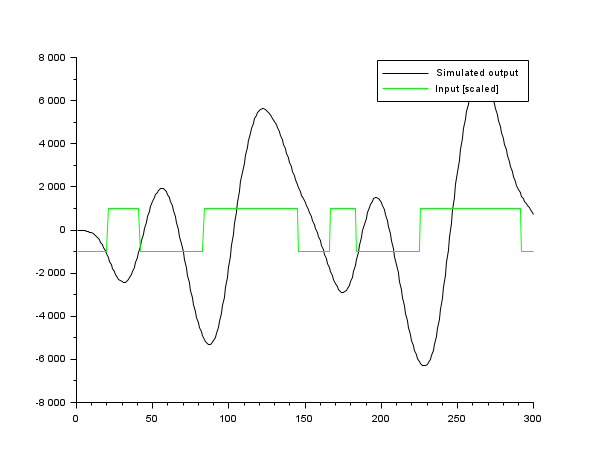
a = [1, -2.851, 2.717, -0.865];
b = [0, 1, 1, 1];
d = [1, 0.7, 0.2];
ar = armac(a, b, d, 1, 1, 1);
disp(_("Simulation of an ARMAX process:"));
disp(ar);
// The input
n = 300;
u = -prbs_a(n, 1, int([2.5,5,10,17.5,20,22,27,35]*100/12));
// simulation
zd = narsimul(ar, u);

// visualization
plot2d(1:n,[zd',1000*u'],style=[1,3]);curves = gce();
legend(["Simulated output";"Input [scaled]"])

See also
| Report an issue | ||
| << arl2 | Identification | armax1 >> |