datafit
Non linear (constrained) parametric fit of measured (weighted) data
Syntax
[p, dmin, status] = datafit(G, Data, p0)
[p, dmin, status] = datafit(G, Data, Wd, p0)
[p, dmin, status] = datafit(G, Data, Wd, 'b', p_inf, p_sup, p0)
[p, dmin, status] = datafit(G, Data, 'b', p_inf, p_sup, p0)
[p, dmin, status] = datafit(G, Data [,Wd] [,Wg][,'b',p_inf,p_sup], p0 [,algo][,stop])
[p, dmin, status] = datafit(G, DG, Data, ..)
[p, dmin, status] = datafit(iprint, ..)
Arguments
- iprint
scalar used to set the trace mode:
Value Action 0 nothing (except errors) is reported 1 initial and final reports 2 adds a report per iteration >2 adds reports on linear search  Most of the reports are displayed in the Scilab console.
- p0
- Matrix of initial guess of the model parameters.
- "b"
- keyword heading the
p_inf, p_supsequence, wherep_infandp_supare real matrices with thep0shape and sizes.p_infis the vector of lower bounds of respectivepcomponents.p_supare upper bounds. - p
- Matrix of the best fitting model parameters, with the
p0sizes. - Data
- (ndc x nd) matrix of experimental data points, where
Data(:,i)are the #nzc coordinates of the ith measurement. - Wd
- Data weights (optional). Row vector with size(Data,2) elements.
- G
Gap function: handle of a function in Scilab language or of a compiled external function. Computed gap(s) between the fitting model and data may be of the first order, not quadratic.
If
G()does not need any input parameters (like constants), only arguments, its syntax must beg = G(p, Data).If
G()needs some input parameters in addition to input arguments, its syntax must beg = G(p, Data, param1, param2, .., paramN). Then,list(G, param1, param2, .., paramN)must be provided todatafit()instead of onlyG.The following definitions will be used:
ng = size(g,1): number of fitting criteria (= of gap definitions).np = size(p,"*"): total number of fitting parameters.nd = size(Data,2): number of data points.ndc = size(Data,1): number of coordinates of each data point.
Then, the sizes of G arguments are the following ones:
g : (ng x nd) matrix - Each column is related to a given data point and retuns its gaps to the fitting model.
- Each row is about a gap definition.
Gmay compute several types of gaps. For instance, the vertical gaps may be returned ing(1,:); the horizontal gaps ing(2,:); the nearest distances ing(3,:); etc.
p : fitting parameters to be optimized. Data : (ndc x nd) matrix: Each column provides the #ndccoordinates of a given data point. IfGcomputes gaps only for a single data point,datafit()will automatically loop over the set ofDatacolumns. This makesdatafit()slower.- DG
- (optional) Handle of a function in Scilab language or of a compiled external
function, computing the partial of
Gwrtp. Its syntax must be likeS = DG(p, Data). The expected sizes of the result are (ng x np x 1) (Data-unvectorized) or (ng x np x nd) (Data-vectorized). - Wg
- Optional (ng x ng) matrix of weights of gaps definitions. Default = eye().
G()defines as many types of gaps as required. Most often, a unique gap will be computed -- most often the vertical one --, but other ones can be computed (horizontal, nearest distance, etc). This matrix allows to weight the different types. - algo
- Word
'qn'(quasi-Newton, default), or'gc'(conjugate gradient), or'nd'(non-differentiable. Thenp_infandp_supparameters bounds are not accepted). Selects the algorithm used to perform the fitting. Seeoptim()for more details. - stop
sequence of optional arguments controlling the convergence of the fitting algorithm:
'ar',nap, [iter [,epsg [,epsf [,epsx]]]], with"ar" reserved keyword heading the list of stopping criteria as defined below. nap maximum number of calls to the cost f function allowed (default: 100). iter maximum number of iterations allowed (default: 100). epsg threshold on gradient norm (default: %eps). epsf threshold controlling the decreasing of f(defined in the description section). Default: 0.epsx threshold controlling the variation of p. This vector (possibly matrix) of same size asp0can be used to scalep. Default: 0.- dmin
- Average Model-to-data residual distance. It is equal to
sqrt(fmin/ng/nd)orsqrt(fmin/ng/sum(Wd)), where fmin is the quadratic residue of the cost functionf(see the description). - status
- return flag = termination status (only for the 'qn' default algorithm.
Set to %nan otherwise):
9is successful. Possible values are:1 : Norm of projected gradient lower than... .... 6 : Optim stops: too small variations in gradient direction. 2 : At last iteration, f decreases by less than... 7 : Stop during calculation of descent direction. 3 : Optim stops: Too small variations for p. 8 : Stop during calculation of estimated hessian. 4 : Optim stops: maximum number of calls to f is reached. 9 : Successful completion. 5 : Optim stops: maximum number of iterations is reached. 10 : Linear search fails.
Other optim() input arguments such that df0,
mem, or 'in' may be used with
datafit(). They will be passed as is to optim().
Description
datafit is used to fit a parametrized model to given data.
A function G(p, Data) must be defined to compute the gaps between the
Data points and a model whose parameters to be tuned are provided
through the matrix p. An initial guess p0
of p values must also be provided.
Starting from initial values p0 of the model parameters,
datafit() varies them in order to minimize the whole Model-to-Data
distance defined as
f = (G(p, Data(:,1))' * Wg * G(p, Data(:,1)))* Wd(1) + ..
    (G(p, Data(:,2))' * Wg * G(p, Data(:,2)))* Wd(2) + ..
    ...
    (G(p, Data(:,nz))' * Wg * G(p,Data(:,nz)))* Wd(nz)
When Wg = eye() (default), this definition is equivalent to
f = sum(G(p, Data(:,1)).^2) * Wd(1) + ..
    sum(G(p, Data(:,2)).^2) * Wd(2) + ..
    ...
    sum(G(p, Data(:,nz)).^2) * Wd(nz)
If in addition G returns only one gap type, this even simplifies to
f = G(p, Data(:,1))^2 * Wd(1) + ..
    G(p, Data(:,2))^2 * Wd(2) + ..
    ...
    G(p, Data(:,nz))^2 * Wd(nz)
datafit() calls optim() to minimize f.
Choosing appropriately p0 may improve and faster
datafit()'s convergence to the best fit.
datafit() checks whether G() is vectorized or not
over Data. If G() works only with a single
data point as a single column of coordinates, then datafit()
loops over data=Data(:,i) points. Otherwise, G(p, Data)
is called for the whole Data array of data coordinates, which is
way faster if G()'s code is truly vectorized.
Examples
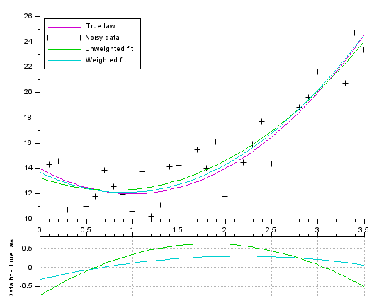
Simple example: Polynomial fitting (parabola = 3 parameters) of weighted data.
Data weights prevent processing this case in a straightforward way with a Vandermonde
matrix and the backslash operator. An initial guess p0 is then
required.
// Model (parabola)
function y=FF(x, p)
    y = (p(1)*x + p(2)).*x + p(3)
endfunction

// Data creation
pa = [2;-4;14] // parameters of the actual law, to generate data
X = 0:0.1:3.5;
Y0 = FF(X, pa);
noise = 5*(rand(Y0)-.5);   // We add some noise
Y = Y0 + noise
Data = [X ; Y];

// Gap function definition
function e=G(p, Data)
    e = Data(2,:) - FF(Data(1,:), p);  // vertical distance
endfunction

// Performing the fitting
// ----------------------
// Without weighting data:
p0 = [1;-1;10]
[p, dmin] = datafit(G, Data, p0);
// The uncertainty is identified to the noise value.
// The weight is set inversely proportional to the uncertainty
[pw, dmin] = datafit(G, Data, 1./abs(noise), p0);

// Display
// -------
scf(0);
clf()
xsetech([0 0 1 0.83])
plot2d(X, Y0, 24)       // True underlaying law
plot2d(X, Y, -1)        // Noisy data
plot2d(X, FF(X, p), 15)  // best unweighted fit
plot2d(X, FF(X, pw), 18) // best weighted fit
legend(["True law" "Noisy data" "Unweighted fit" "Weighted fit"],2)

xsetech([0 .75 1 0.25])
plot2d(X, FF(X,p)-Y0, 15)  // remaining gap <= best unweighted fit
plot2d(X, FF(X,pw)-Y0, 18) // remaining gap <= best weighted fit
ylabel("Data fit - True law")
ax = gca(); ax.x_location = "top";
tmp = ax.x_ticks.labels;
gca().x_ticks.labels = emptystr(size(tmp,"*"),1);
xgrid(color("grey70"))
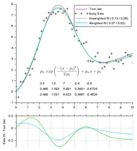
Fitting a gaussian curve + sloping base (5 parameters):
function Y=model(P, X)
    Y = P(3) * exp(-(X-P(1)).^2 / (2*P(2)*P(2))) + P(4)*X + P(5);
endfunction
// -------------------------------
// Gap function
function r=gap(P, XY)
    r = XY(2,:) - model(P,XY(1,:))
endfunction
// -------------------------------
// True parameters
Pg = [3.5 1.5 7 0.4 -0.5]; // mean stDev ymax a(.x) b

// Generating data
// ---------------
X = 0:0.2:10;
Np = length(X);
Y0 = model(Pg, X);              // True law
noise = (rand(Y0)-.5)*Pg(3)/4;
Y = Y0 + noise                  // Noised data
Data = [X ; Y];

// Trying to recover original parameters from the (noisy) data:
// -----------------------------------------------------------
// Performing the fitting = parameters optimization
[v, k] = max(Y0);
P0 = [X(k) 1 v 1 1];
[P, dmin, s]  = datafit(gap, Data, P0);
Wd =  1./abs(noise);
[Pw, dminw, s] = datafit(gap, Data, Wd, P0);

// Computing fitting curves from found parameters
fY = model(P, X);
fYw = model(Pw, X);

// Display
// -------
scf(0);
clf()
xsetech([0 0 1 0.8])
plot2d(X, Y0, 24)  // True underlaying law
plot2d(X, Y,  -1)  // Noisy data
plot2d(X, fY, 15)  // best unweighted fit
plot2d(X, fYw,18)  // best weighted fit

// Legends: Average vertical Model-Data distance:
// True one v/s according to the residual cost
L_1 = "Unweighted fit (%5.2f /%5.2f)";
L_1 = msprintf(L_1, mean(abs(fY-Y0)), sqrt(dmin/Np));
L_2 = "Weighted fit (%5.2f /%5.2f)";
L_2 = msprintf(L_2, mean(abs(fYw-Y0)), sqrt(dminw/sum(Wd)));
legend(["True law", "Noisy Data", L_1, L_2],1)

// Params: row#1: true params row#2:
//  from unweighted fit row#3: from weighted fit
[xs, ys] = meshgrid(linspace(2,6,5), linspace(0.5,-0.5,3));
xnumb(xs, ys, [Pg ; P ; Pw]);
LawTxt = "$\Large p_3\,.\,"+..
         "exp\left({-(x-p_1)^2}\over{2\,p_2} \right)+p_4.x+p_5$";
xstring(2, 1.3, LawTxt)

// Plotting residus:
xsetech([0 .75 1 0.25])
plot2d(X, model(P ,X)-Y0, 15) // remaining gap with best unweighted fit
plot2d(X, model(Pw,X)-Y0, 18) // remaining gap best weighted fit
ylabel("Data fit - True law")
ax = gca();
ax.x_location = "top";
gca().x_ticks.labels = emptystr(size(ax.x_ticks.labels, "*"),1);
xgrid(color("grey70"))
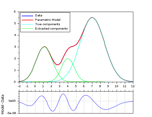
Extraction of 3 overlapping gaussian curves (9 parameters): example with constrained bounds and a matrix of parameters.
// Basic gaussian component:
function Y=gauss(X, average, stDev, ymax)
    Y = ymax * exp(-(X-average).^2 / (2*stDev*stDev))
endfunction

// Model: cumulated gaussian laws
function r=model(P, X)
    // P(1,:): averages  P(2,:): standard deviation  P(3,:): ymax
    r = 0;
    for i = 1:size(P,2)
        r = r + gauss(X, P(1,i), P(2,i), P(3,i));
    end
endfunction

// Gap function:
function r=gap(P, XY)
    r = XY(2,:) - model(P, XY(1,:))
endfunction

// True parameters :
Pa = [ 1.1  4    7    // averages
        1  0.8  1.5   // standard deviations
        3   2   5.5   // ymax
     ];
Nc = size(Pa,2);      // Number of summed curves
Np = 200;             // Number of data points

// Data generation (without noise)
xmin = 0;
xmax = 10;
X = linspace(xmin-2, xmax+2, Np);
Y = model(Pa, X);
Data = [X ; Y];      // Curve to analyze / fit

// FITTING
// -------
// Fitting parameters: initial values and bounds (amplitudes must be > 0)
Po = [ linspace(xmin,xmax,Nc) ; ones(1,Nc)*0.5 ; ones(1,Nc)*max(Y)/2];
Pinf = [ones(1,Nc)*-2 ; ones(1,Nc)*0.1 ; ones(1,Nc)*1];
Psup = [ones(1,Nc)*12 ; ones(1,Nc)*3   ; ones(1,Nc)*max(Y)*1.2];
// Fitting
[P, dmin] = datafit(gap, Data, 'b',Pinf,Psup, Po, 'qn','ar',200,200);

// Display
// -------
clf()
xsetech([0 0 1 0.8]);
plot(X, Y, "-b", X, model(P,X), "-r");
gca().children.children(1:2).thickness = 2;
for i = 1:Nc
plot(X, gauss(X, Pa(1,i), Pa(2,i), Pa(3,i)), "-c"); // True gaussian components
plot(X, gauss(X, P(1,i), P(2,i), P(3,i)), "-g");    // Extracted gaussian components
end
legend("Data", "Parametric Model","True components", "Extracted components",  2);

xsetech([0 0.75 1 0.25])
plot(X, model(P,X)-Y);
gca().x_location = "top";
gca().x_ticks.labels = emptystr(size(gca().x_ticks.labels,"*"),1);
ylabel("Model - Data")
xgrid(color("grey70"))
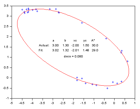
With a parametric curve: Fitting a off-centered tilted 2D elliptical arc (5 parameters).
function g=Gap(p, Data)
    // p: a, b, center xc, yc, alpha tilt °
    C = cosd(p(5)); S = -sind(p(5));
    x = Data(1,:) - p(3);
    y = Data(2,:) - p(4);
    g = ((x*C - y*S )/p(1)).^2 + ((x*S + y*C)/p(2)).^2 - 1;
endfunction

// Generating the data
// -------------------
// Actual parameters :
Pa = [3, 1.3, -2, 1.5, 30];
Np = 30;            // Number of data points
Theta = grand(1,Np, "unf",-100, 170);
// untilted centered noisy arc
x = Pa(1)*(cosd(Theta) + grand(Theta, "unf", -0.07, 0.07));
y = Pa(2)*(sind(Theta) + grand(Theta, "unf", -0.07, 0.07));
// Tilting and off-centering the arc
A = Pa(5);
C = cosd(A); S = sind(A);
xe =  C*x + y*S + Pa(3);
ye = -S*x + y*C + Pa(4);
Data = [xe ; ye];

// Retrieving parameters from noisy data
// -------------------------------------
// Initial estimation
ab0 = (strange(xe)+strange(ye))/2;
xc0 = mean(xe);
yc0 = mean(ye);
A0 = -atand(reglin(xe,ye));
P0 = [ab0 ab0/2 xc0 yc0 A0];
// Parameters bounds
Pinf = [ 0     0     xc0-2*ab0, yc0-2*ab0 -90];
Psup = [3*ab0 3*ab0  xc0+2*ab0, yc0+2*ab0  90];// Fitting

// FITTING
[P, dmin] = datafit(Gap, Data, 'b',Pinf,Psup, P0);

// P(1) is the longest axis:
if P(1)<P(2) then
    P([1 2]) = P([2 1]);
    P(5) = 90 - P(5);
end

// DISPLAY
// -------
disp([Pa;P], dmin);
// A successful fit should lead to dmin ~ noise amplitude

clf
plot(xe, ye, "+")   // Data
// Model
Theta = 0:2:360;
x = P(1) * cosd(Theta);
y = P(2) * sind(Theta);
A = P(5);
[x, y] = (x*cosd(A)+y*sind(A)+P(3), -x*sind(A)+y*cosd(A)+P(4));
plot(x, y, "r")
isoview
// Parameters values:
Patxt = msprintf("%5.2f   %5.2f   %5.2f   %5.2f  %5.1f", Pa);
Ptxt  = msprintf("%5.2f   %5.2f   %5.2f   %5.2f  %5.1f", P);
xstring(-3.7, 1.2, ["" "    a           b        xc       yc     A°"
                    "Actual:" Patxt
                    "Fit:" Ptxt ])
xstring(-2.5, 0.9, "dmin = " + msprintf("%5.3f", dmin))
See also
History
| Version | Description |
| 6.1 |
|
| Report an issue | ||
| << Nonlinear Least Squares | Nonlinear Least Squares | leastsq >> |