Please note that the recommended version of Scilab is 2026.1.0. This page might be outdated.
See the recommended documentation of this function
csim
simulation (time response) of linear system
Syntax
[y [,x]]=csim(u,t,sl,[x0 [,tol]])
Arguments
- u
function, list or string (control)
- t
real vector specifying times with,
t(1)is the initial time (x0=x(t(1))).- sl
A SISO or SIMO linear dynamical system, in state space, transfer function or zpk representations, in continuous time.
- y
a matrix such that
y=[y(t(i)], i=1,..,n- x
a matrix such that
x=[x(t(i)], i=1,..,n- tol
a 2 vector [atol rtol] defining absolute and relative tolerances for ode solver (see ode)
Description
simulation of the controlled linear system sl.
sl is assumed to be a continuous-time system
represented by a syslin list.
u is the control and x0 the initial state.
y is the output and x the state.
The control can be:
1. a function : [inputs]=u(t)
2. a list : list(ut,parameter1,....,parametern) such that:
inputs=ut(t,parameter1,....,parametern) (ut is a function)
3. the string "impuls" for impulse
response calculation (here sl must have
a single input and x0=0). For systems
with direct feedthrough, the infinite pulse at t=0 is
ignored.
4. the string "step" for step response calculation
(here sl must have a single input and
x0=0)
5. a vector giving the values of u corresponding to each t value.
Examples
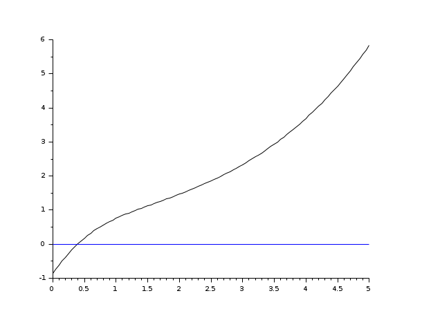
s=poly(0,'s');
rand('seed',0);
w=ssrand(1,1,3);
w('A')=w('A')-2*eye();
t=0:0.05:5;
//impulse(w) = step (s * w)
plot2d([t',t'],[(csim('step',t,tf2ss(s)*w))',0*t'])
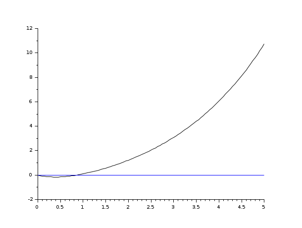
s=poly(0,'s');
rand('seed',0);
w=ssrand(1,1,3);
w('A')=w('A')-2*eye();
t=0:0.05:5;
plot2d([t',t'],[(csim('impulse',t,w))',0*t'])

s=poly(0,'s');
rand('seed',0);
w=ssrand(1,1,3);
w('A')=w('A')-2*eye();
t=0:0.05:5;
//step(w) = impulse (s^-1 * w)
plot2d([t',t'],[(csim('step',t,w))',0*t'])
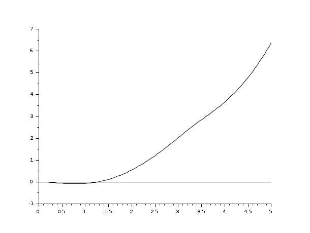
s=poly(0,'s');
rand('seed',0);
w=ssrand(1,1,3);
w('A')=w('A')-2*eye();
t=0:0.05:5;
plot2d([t',t'],[(csim('impulse',t,tf2ss(1/s)*w))',0*t'])

s=poly(0,'s');
rand('seed',0);
w=ssrand(1,1,3);
w('A')=w('A')-2*eye();
t=0:0.05:5;
//input defined by a time function
deff('u=timefun(t)','u=abs(sin(t))')
clf();plot2d([t',t'],[(csim(timefun,t,w))',0*t'])
See also
- syslin — linear system definition
- dsimul — state space discrete time simulation
- flts — time response (discrete time, sampled system)
- ltitr — discrete time response (state space)
- rtitr — discrete time response (transfer matrix)
- ode — ordinary differential equation solver
- impl — differential algebraic equation
History
| Version | Description |
| 6.0 | handling zpk representation |
| Report an issue | ||
| << arsimul | Time Domain | damp >> |