Please note that the recommended version of Scilab is 2026.1.0. This page might be outdated.
See the recommended documentation of this function
odedc
discrete/continuous ode solver
Calling Sequence
yt=odedc(y0,nd,stdel,t0,t,f)
Arguments
- y0
a real column vector (initial conditions),
y0=[y0c;y0d]wherey0dhasndcomponents.- nd
an integer, dimension of
y0d- stdel
a real vector with one or two entries,
stdel=[h, delta](withdelta=0as default value).- t0
a real scalar (initial time).
- t
a real (row) vector, instants where
ytis calculated.- f
an external i.e. a function or a character string or a list with calling sequence:
yp=f(t,yc,yd,flag).- f
an external i.e. a function or a character string or a list with calling sequence:
yp=f(t,yc,yd,flag)- a list
This form of external is used to pass parameters to the function. It must be as follows:
list(f, p1, p2,...)
where the calling sequence of the function
fis nowyp = f(t, yc, yd, flag, p1, p2,...)
fstill returns the function value as a function of(t, yc, yd, flag, p1, p2,...), andp1, p2,...are function parameters.- a character string
it must refer to the name of a C or fortran routine, assuming that <
f_name> is the given name.The Fortran calling sequence must be
<f_name>(iflag, nc, nd, t, y, ydp)double precision t, y(*), ydp(*)integer iflag, nc, ndThe C calling sequence must be
void <f_name> (int *iflag, int *nc,
                                                int *nd, double *t, double *y, double *ydp)
In both Fortran and C cases, the input arguments are:
iflag=0or1nc= number of continuous statesycnd= number of discrete statesydt= timey=[yc; yd; param]. param may be used to get extra arguments which have been given in the odedc call(y = odedc([y0c; y0d], nd, stdel, t0, t, list('fexcd', param)))As output
ydp, the routine must computeydp[0:nc-1]) = d/dt ( yc(t) )foriflag=0andydp[0:nd-1] = yd(t+)foriflag=1.
Description
y=odedc([y0c;y0d],nd,[h,delta],t0,t,f) computes
the solution of a mixed discrete/continuous system. The discrete system
state yd_k is embedded into a piecewise constant
yd(t) time function as follows:
yd(t) = yd_k for t in
[t_k=delay+k*h,t_(k+1)=delay+(k+1)*h] (with delay=h*delta).
The simulated equations are now:
dyc/dt = f(t,yc(t),yd(t),0),  for t in [t_k,t_(k+1)]
yc(t0) = y0c
and at instants t_k the discrete variable
yd is updated by:
yd(t_k+) = f(yc(t_k-),yd(t_k-),1)
Note that, using the definition of yd(t) the last
equation gives
yd_k = f (t_k,yc(t_k-),yd(t_(k-1)),1) (yc is time-continuous: yc(t_k-)=yc(tk))
The calling parameters of f are fixed:
ycd=f(t,yc,yd,flag); this function must return either
the derivative of the vector yc if
flag=0 or the update of yd if
flag=1.
ycd=dot(yc) must be a vector with same dimension
as yc if flag=0 and
ycd=update(yd) must be a vector with same dimension as
yd if flag=1.
t is a vector of instants where the solution
y is computed.
y is the vector
y=[y(t(1)),y(t(2)),...].
This function can be called with the same optional parameters as the ode
function (provided nd and stdel are given in
the calling sequence as second and third parameters). In particular
integration flags, tolerances can be set. Optional parameters can be set
by the odeoptions function.
An example for calling an external routine is given in
SCIDIR/default/fydot2.f
External routines can be dynamically linked (see
link).
Examples
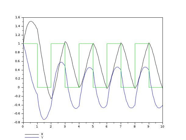
//Linear system with switching input
deff('xdu=phis(t,x,u,flag)','if flag==0 then xdu=A*x+B*u; else xdu=1-u;end');
x0=[1;1];
A=[-1,2;-2,-1];
B=[1;2];
u=0;
nu=1;
stdel=[1,0];
u0=0;
t=0:0.05:10;
xu=odedc([x0;u0],nu,stdel,0,t,phis);
x=xu(1:2,:);
u=xu(3,:);
nx=2;
plot2d1('onn',t',x',[1:nx],'161');
plot2d2('onn',t',u',[nx+1:nx+nu],'000');
//Fortran external (see fydot2.f):
norm(xu-odedc([x0;u0],nu,stdel,0,t,'phis'),1)
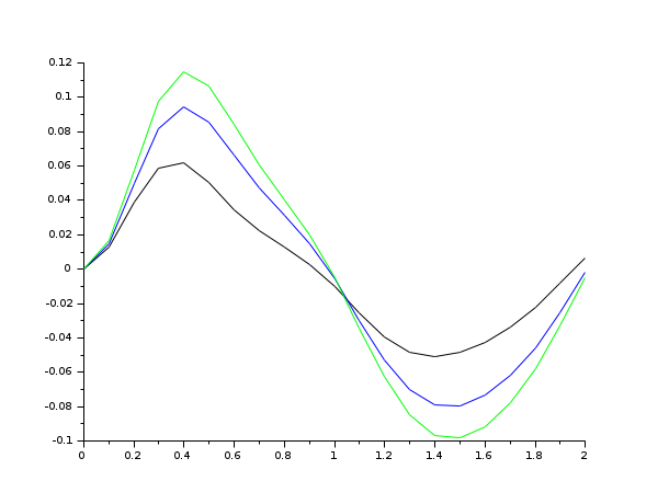
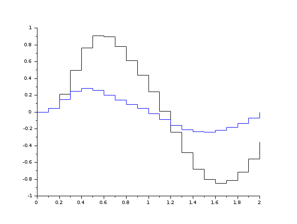
//Sampled feedback
//
//        |     xcdot=fc(t,xc,u)
//  (system)   |
//        |     y=hc(t,xc)
//
//
//        |     xd+=fd(xd,y)
//  (feedback) |
//        |     u=hd(t,xd)
//
deff('xcd=f(t,xc,xd,iflag)',...
  ['if iflag==0 then '
   '  xcd=fc(t,xc,e(t)-hd(t,xd));'
   'else '
   '  xcd=fd(xd,hc(t,xc));'
   'end']);
A=[-10,2,3;4,-10,6;7,8,-10];
B=[1;1;1];
C=[1,1,1];
Ad=[1/2,1;0,1/20];
Bd=[1;1];
Cd=[1,1];
deff('st=e(t)','st=sin(3*t)')
deff('xdot=fc(t,x,u)','xdot=A*x+B*u')
deff('y=hc(t,x)','y=C*x')
deff('xp=fd(x,y)','xp=Ad*x + Bd*y')
deff('u=hd(t,x)','u=Cd*x')
h=0.1;t0=0;t=0:0.1:2;
x0c=[0;0;0];
x0d=[0;0];
nd=2;
xcd=odedc([x0c;x0d],nd,h,t0,t,f);
norm(xcd-odedc([x0c;x0d],nd,h,t0,t,'fcd1')) // Fast calculation (see fydot2.f)
plot2d([t',t',t'],xcd(1:3,:)');
xset("window",2);
plot2d2("gnn",[t',t'],xcd(4:5,:)');
xset("window",0);
See Also
- ode — ordinary differential equation solver
- link — dynamic linker
- odeoptions — set options for ode solvers
- csim — simulation (time response) of linear system
- external — Scilab Object, external function or routine
| Report an issue | ||
| << ode_root | Differential calculus, Integration | odeoptions >> |